
Name:
Class:
Date:
chapter 8
Answer Key

Name:
Class:
Date:
chapter 8
30. b
31. b
32. a
33. d
34. c
35. d
36. d
37. d
38. a
39. a
40. a
41. a
42. d
43. b
44. c
45. b
46. b
47. a
48. c
49. d
50. c
51. a

chapter 8
52. d
53. c
54. b
55.
(A)
56.
57.
0.53 ± 0.0489 = (0.4811, 0.5789).
Since confidence interval ranges from about 48% to 57.9%, it is difficult to conclude that a majority of people favors Coke. It could be
below 50%.
0.53 ± 0.0219 = (0.5081, .5519).
In this case the 95% confidence interval is entirely above 50%, the data is now more convincing than it was previously.
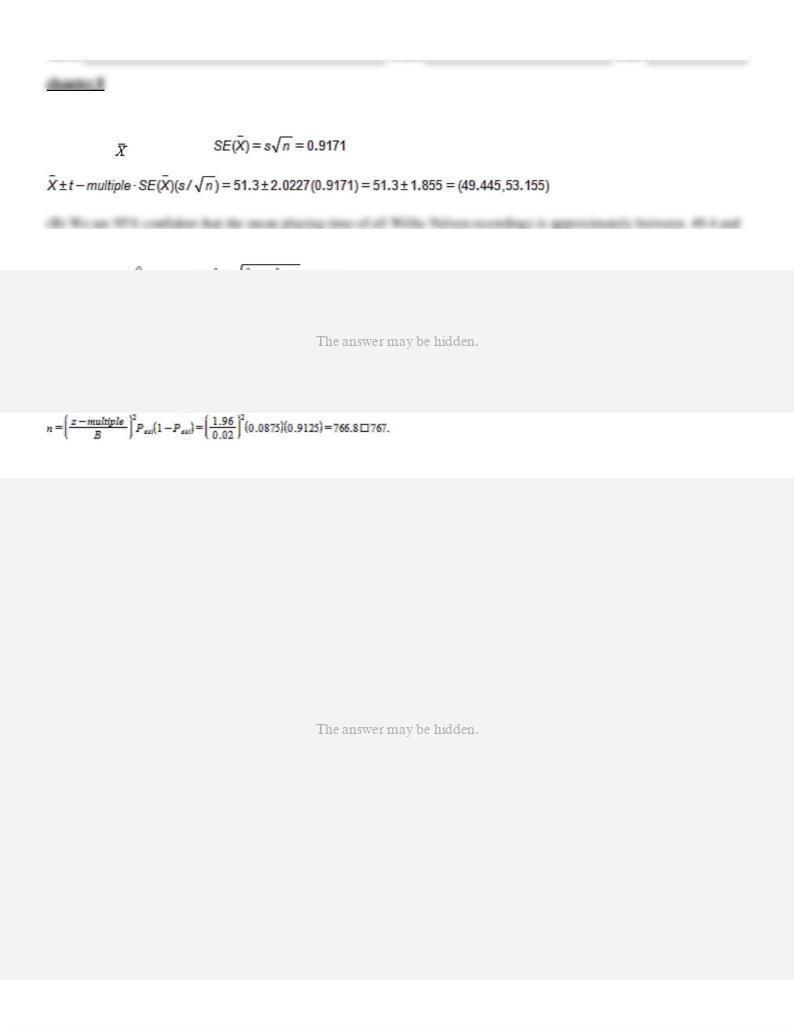
(C) = 0.53, z – multiple = 1.96, B = .01. The sample size for proportion is given by:
.

Name:
Class:
Date:
chapter 8
58.
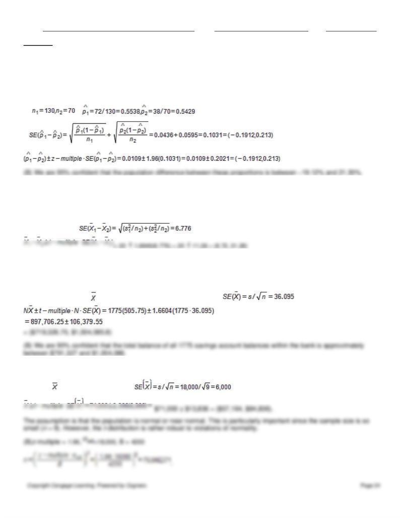
(B) The store can be 95% confident that the typical average annual balance of all 15,000 credit card accounts will be
somewhere between $210.84 and $220.66.
(C) The point estimate of the total of the annual credit account balances is 15,000 ($215.75)=$3,236,250. Similarly, the
upper and lower confidence interval limits for the total are 15,000($210.84)=$3,162,575 and 15,000($220.66) =
$3,309,925, respectively. The store’s current administrative costs ($1,000,000) are over 30% of the best possible case for
the total of the average annual account balances (the upper limit of the interval, $3,309,925), therefore the credit card
program is not worthwhile.
59.
.
60.
61.
62.
(A) We applied the paired sample analysis with , where: D = Difference = Appraised value –
Name:
Class:
Date:
63.
(A) n = 10, = 51.3, s = 5.8,
53.2 minutes.

Name:
Class:
Date:
66.
(A) By using the Excel function = TDIST (2, 15, 1) we get 0.03197.
(B) By using the Excel function = TDIST (2, 150, 1) we get 0.02365.
(C) The smaller the degrees of freedom, the larger the variance of t, and so the larger the tail probabilities are.
(D) By using the Excel function = 1 – NORMDIST (2) we get 0.02275.
Name:
Class:
Date:
chapter 8
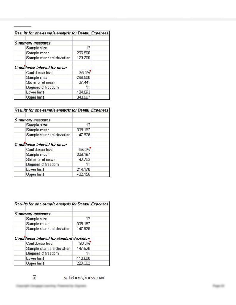
(E)
The additional $500 in dental expenses, divided across the sample of 12, raises the mean by $41.67
and increases the standard deviation by nearly $18.20. The interval width increases over $23 in the
process.
(F)
68.
(A) n = 40, = 1250, s = 350,

Name:
Class:
Date:
chapter 8
(B) z – multiple = 1.96, = 350, B = 100. Then,
69.
(A)
= (0.1675), 0.5125)
70.
71.
.
72.
0.8334
74.
= 0.25, z – multiple = 2.575, B = 0.02
Name:
Class:
Date:
chapter 8
75.
- 1.7531 and + 1.7531
76.
(A) ,
=
77.
0.8182
78.
t-multiple = 1.6646,
79.
- 2.1315 and + 2.1315
80.
(A) N = 1775, n = 100, = 505.75, s = 360.95, t – multiple = 1.6604,
81.
(A) n = 9, = 71,000, s = 18,000. Then
Name:
Class:
Date:
chapter 8
82.
(A) n = 100,
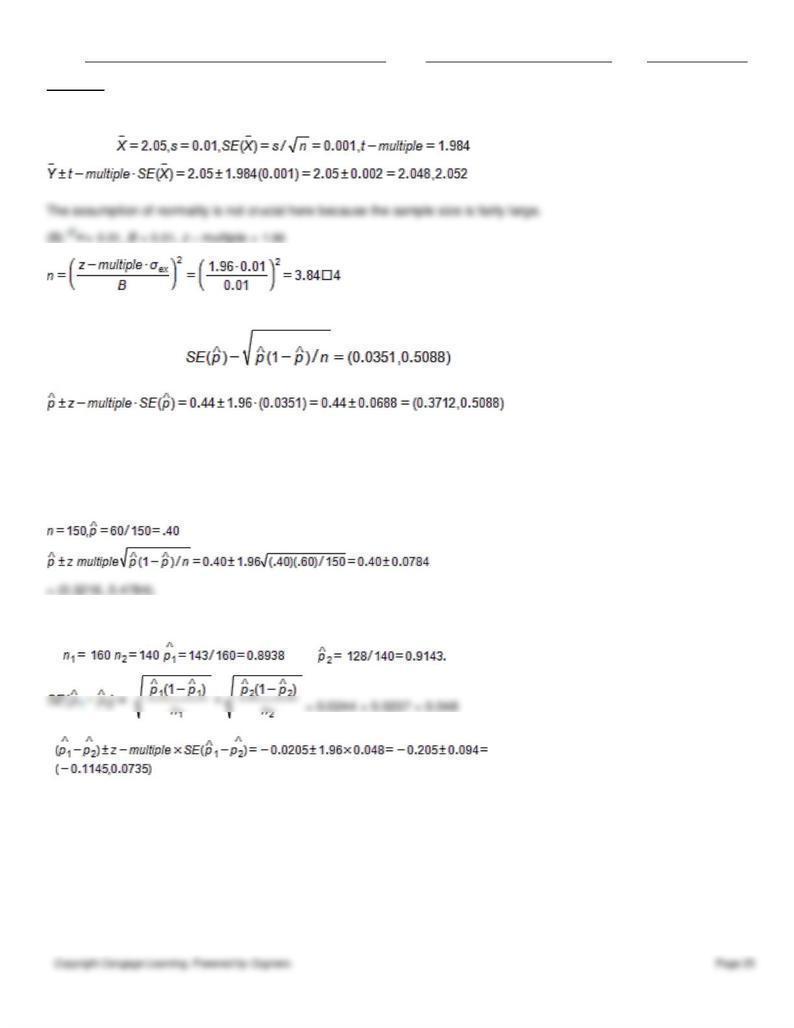
83. (A)= 88/200 = 0.44, z – multiple = 1.96
(B) The dealer can infer that the proportion of all customers who still own the cars they purchased at the dealership 6
years earlier is somewhere between 03712 and 0.5088 with a 95% level of confidence.
84.
85.
(A , , , and
(B) We are 95% confident that the population difference between these proportions is between –0.1147 and 0.0736.
Since the interval includes both negative differences and positive differences, the company really cannot conclude
whether one form of training is better than the other or vice-versa.
86.
0.1244