
Chapter 36 Extending the Analysis of Aggregate Supply Answer Key
Multiple Choice Questions
1.
In terms of aggregate supply, a period in which nominal wages and other resource prices
are unresponsive to price-level changes is called the:
AACSB: Analytic
Accessibility: Keyboard Navigation
Blooms: Remember
Difficulty: 1 Easy
Learning Objective: 36-01 Explain the relationship between short-run aggregate supply and long-run aggregate supply.
Topic: From short run to long run
2.
In terms of aggregate supply, a period in which nominal wages and other resource prices
are fully responsive to price-level changes is called the:
AACSB: Analytic
Accessibility: Keyboard Navigation
Blooms: Remember
Difficulty: 1 Easy
Learning Objective: 36-01 Explain the relationship between short-run aggregate supply and long-run aggregate supply.
Topic: From short run to long run

3.
In the extended analysis of aggregate supply, the short-run aggregate supply curve is:
AACSB: Analytic
Accessibility: Keyboard Navigation
Blooms: Remember
Difficulty: 1 Easy
Learning Objective: 36-01 Explain the relationship between short-run aggregate supply and long-run aggregate supply.
Topic: From short run to long run
4.
In terms of aggregate supply, the short run is a period in which:
AACSB: Analytic
Accessibility: Keyboard Navigation
Blooms: Remember
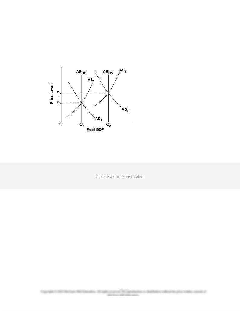
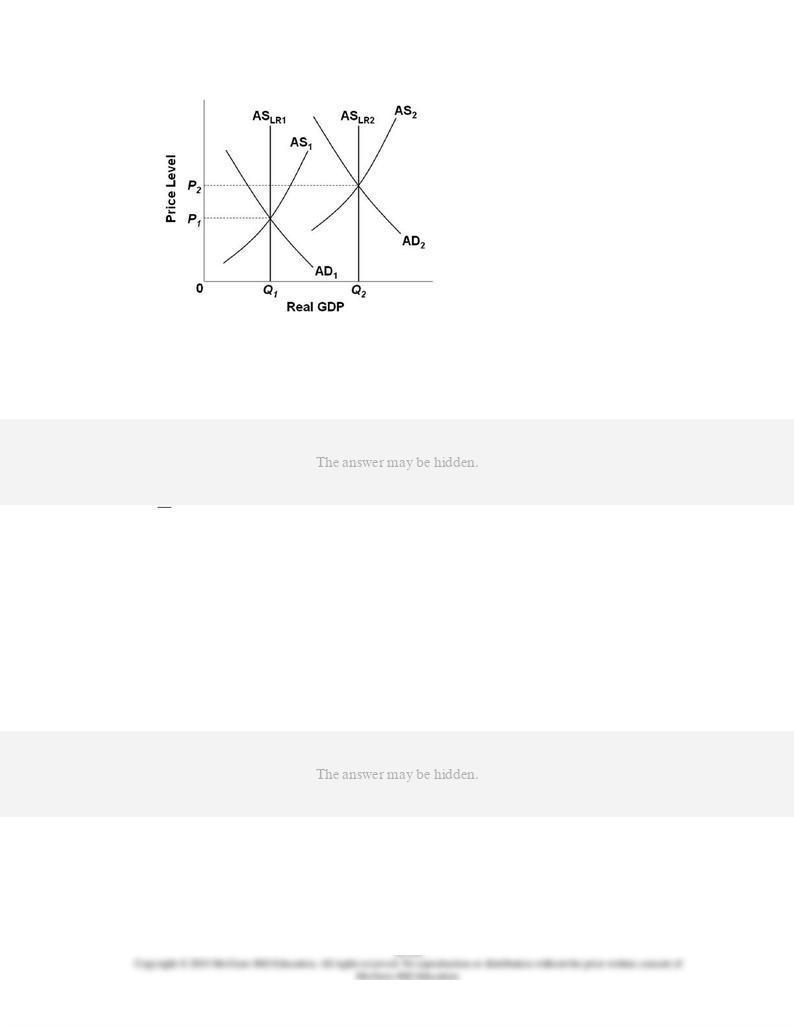
Difficulty: 1 Easy
Learning Objective: 36-01 Explain the relationship between short-run aggregate supply and long-run aggregate supply.
Topic: From short run to long run
5.
In terms of aggregate supply, the
difference
between the long run and the short run is that
in the long run:
AACSB: Analytic
Accessibility: Keyboard Navigation
Blooms: Remember

Difficulty: 1 Easy
Learning Objective: 36-01 Explain the relationship between short-run aggregate supply and long-run aggregate supply.
Topic: From short run to long run
6.
The long-run aggregate supply curve is vertical:
AACSB: Reflective Thinking
Accessibility: Keyboard Navigation
Blooms: Understand
Difficulty: 2 Medium
Learning Objective: 36-01 Explain the relationship between short-run aggregate supply and long-run aggregate supply.
Topic: From short run to long run
7.
The short-run aggregate supply curve is upsloping because higher price levels:
AACSB: Reflective Thinking
Accessibility: Keyboard Navigation
Blooms: Understand
Difficulty: 2 Medium
Learning Objective: 36-01 Explain the relationship between short-run aggregate supply and long-run aggregate supply.
Topic: From short run to long run
8.
Other things equal, a decrease in the price level will:
AACSB: Reflective Thinking
Accessibility: Keyboard Navigation
Blooms: Understand
Difficulty: 2 Medium
Learning Objective: 36-01 Explain the relationship between short-run aggregate supply and long-run aggregate supply.
Topic: From short run to long run
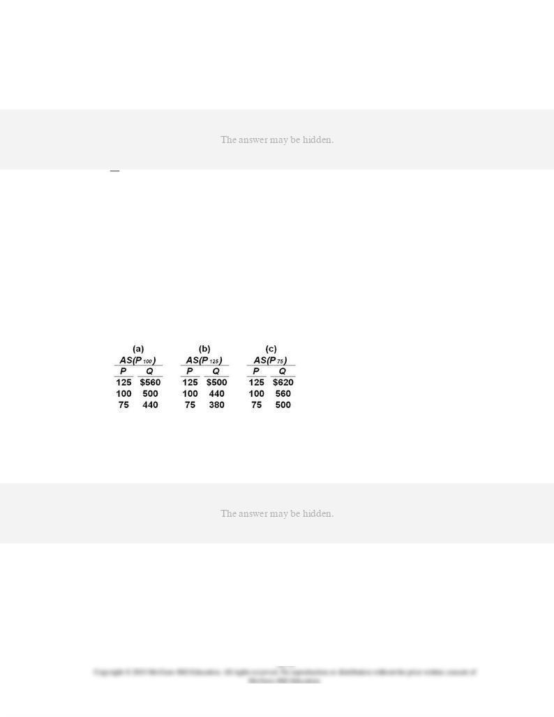
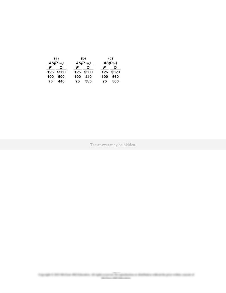
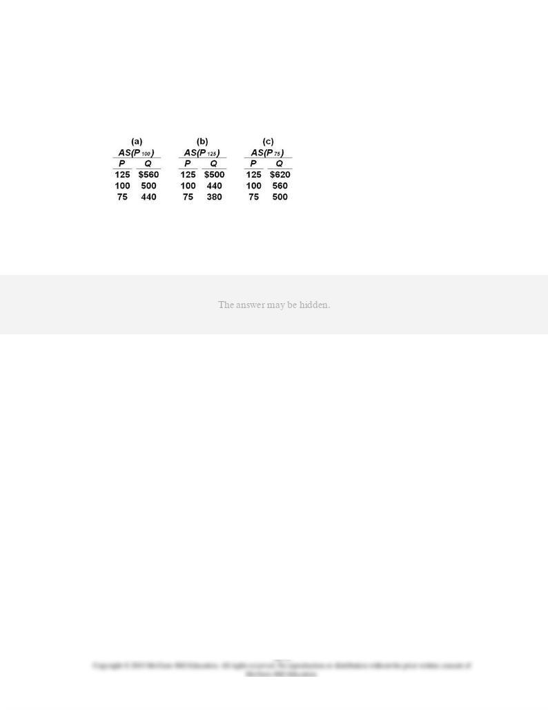
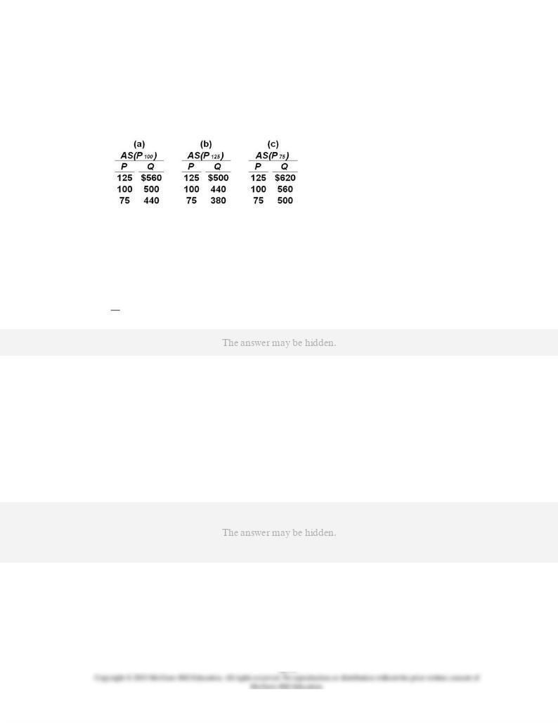
9.
Suppose the full employment level of real output (
Q
) for a hypothetical economy is $500,
the price level (
P
) initially is 100, and prices and wages are flexible both upward and
downward. Use the following short-run aggregate supply schedules to answer the
question.
Refer to the information given. If the price level unexpectedly increases from 100 to 125,
the level of real output in the short run will:
AACSB: Analytic
Blooms: Analyze
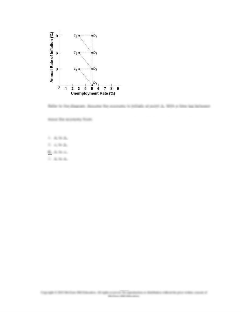
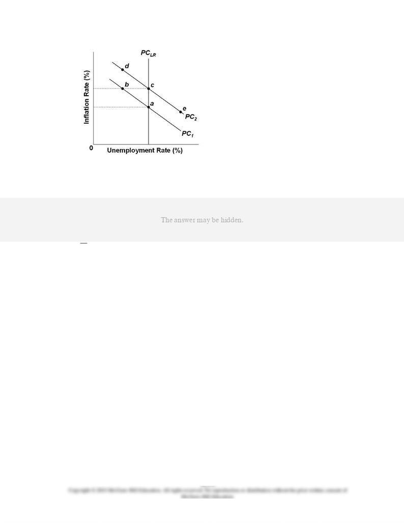
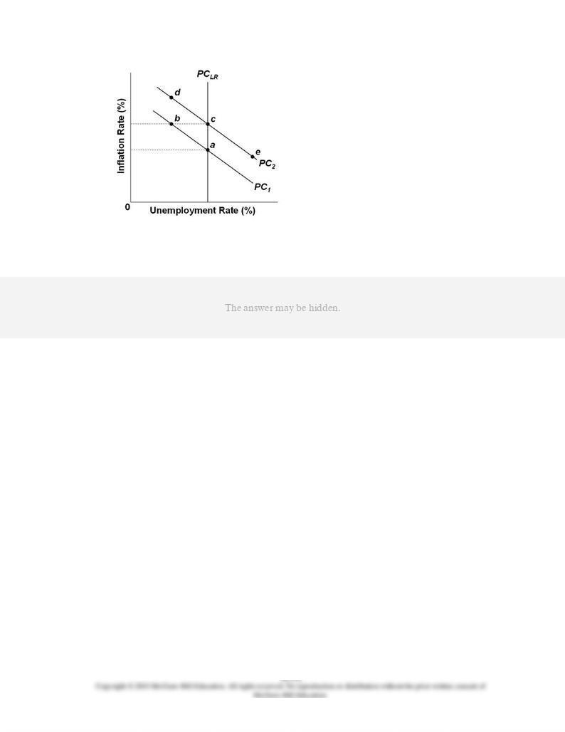
Difficulty: 3 Hard
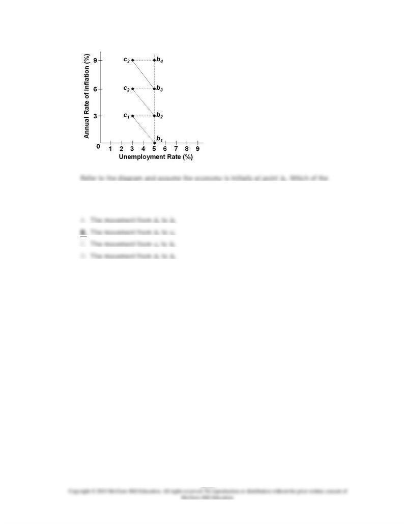
Learning Objective: 36-01 Explain the relationship between short-run aggregate supply and long-run aggregate supply.
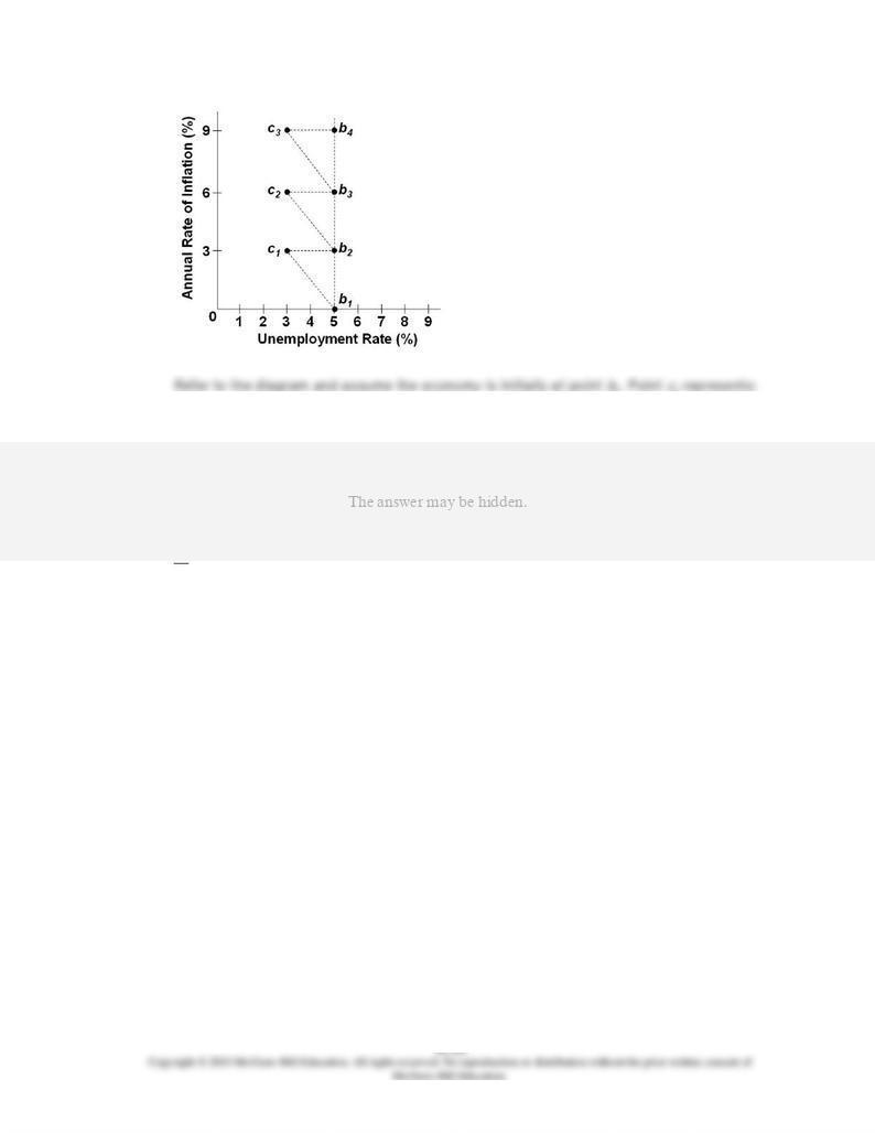
Topic: From short run to long run
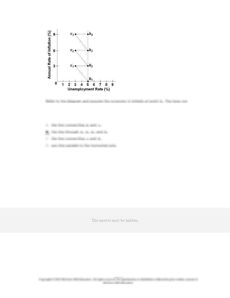
Type: Table
10.
Suppose the full employment level of real output (
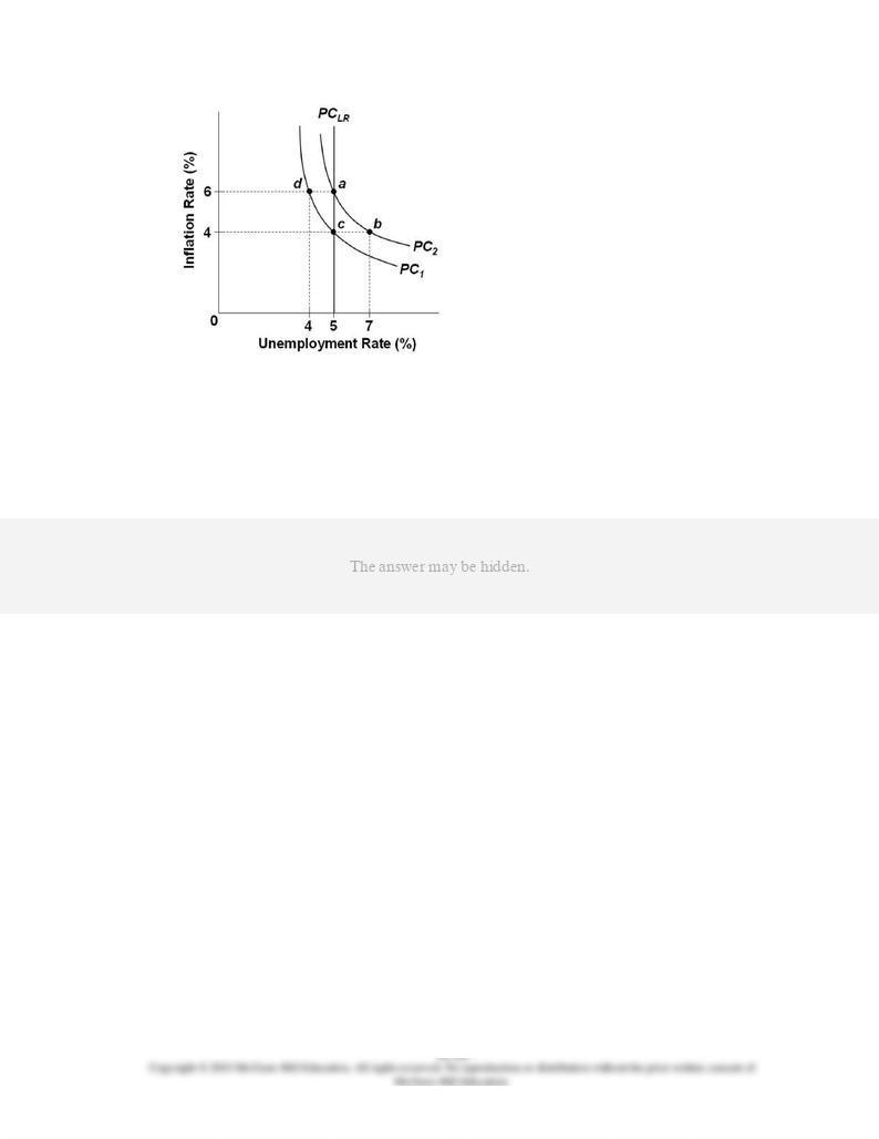
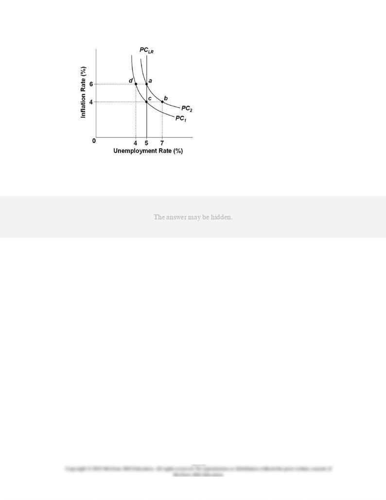
Q
) for a hypothetical economy is $500,
the price level (
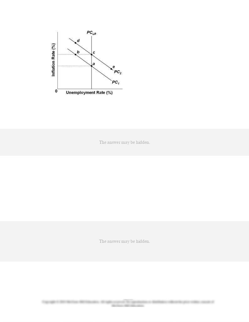
P
) initially is 100, and prices and wages are flexible both upward and
downward. Use the following short-run aggregate supply schedules to answer the
question.
Refer to the information given. In the long run, an increase in the price level from 100 to
125 will:
A.
increase real output from $500 to $560.
B.
decrease real output from $500 to $440.
C.
change the aggregate supply schedule from (a) to (c) and result in an equilibrium level
of real output of $560.
AACSB: Analytic
Blooms: Analyze
Difficulty: 3 Hard
Learning Objective: 36-01 Explain the relationship between short-run aggregate supply and long-run aggregate supply.
Topic: From short run to long run
Type: Table
11.
Suppose the full employment level of real output (
Q
) for a hypothetical economy is $500,
the price level (
P
) initially is 100, and prices and wages are flexible both upward and
downward. Use the following short-run aggregate supply schedules to answer the
question.
Refer to the information given. If the price level unexpectedly declines from 100 to 75, the
level of real output in the short run will:
AACSB: Analytic
Blooms: Analyze
Difficulty: 3 Hard
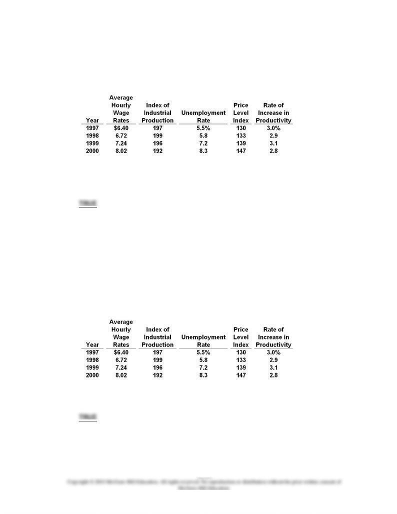
Learning Objective: 36-01 Explain the relationship between short-run aggregate supply and long-run aggregate supply.
Topic: From short run to long run
Type: Table
12.
Suppose the full employment level of real output (
Q
) for a hypothetical economy is $500,
the price level (
P
) initially is 100, and prices and wages are flexible both upward and
downward. Use the following short-run aggregate supply schedules to answer the
question.
Refer to the information given. In the long run, a fall in the price level from 100 to 75 will:
A.
decrease real output from $500 to $440.
B.
increase real output from $500 to $620.
C.
change the aggregate supply schedule from (a) to (c) and produce an equilibrium level
of real output of $500.
AACSB: Analytic
Blooms: Analyze
Difficulty: 3 Hard
Learning Objective: 36-01 Explain the relationship between short-run aggregate supply and long-run aggregate supply.
Topic: From short run to long run
Type: Table
13.
Which of the following statements is true?
AACSB: Analytic
Accessibility: Keyboard Navigation
Blooms: Remember
Difficulty: 1 Easy
Learning Objective: 36-01 Explain the relationship between short-run aggregate supply and long-run aggregate supply.
Topic: From short run to long run
14.
1 to
2.
C.
change aggregate supply from AS2 to AS1.
2.
AACSB: Reflective Thinking
Blooms: Analyze
Difficulty: 3 Hard
Learning Objective: 36-01 Explain the relationship between short-run aggregate supply and long-run aggregate supply.
Topic: From short run to long run
Type: Graph
15.
2.
B.
change aggregate supply from AS2 to AS1.
2 to
1.
AACSB: Reflective Thinking
Blooms: Analyze
Difficulty: 3 Hard
Learning Objective: 36-01 Explain the relationship between short-run aggregate supply and long-run aggregate supply.
Topic: From short run to long run
Type: Graph
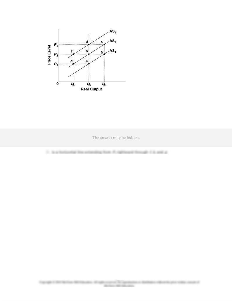
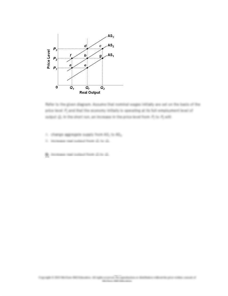
16.
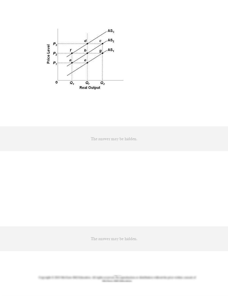
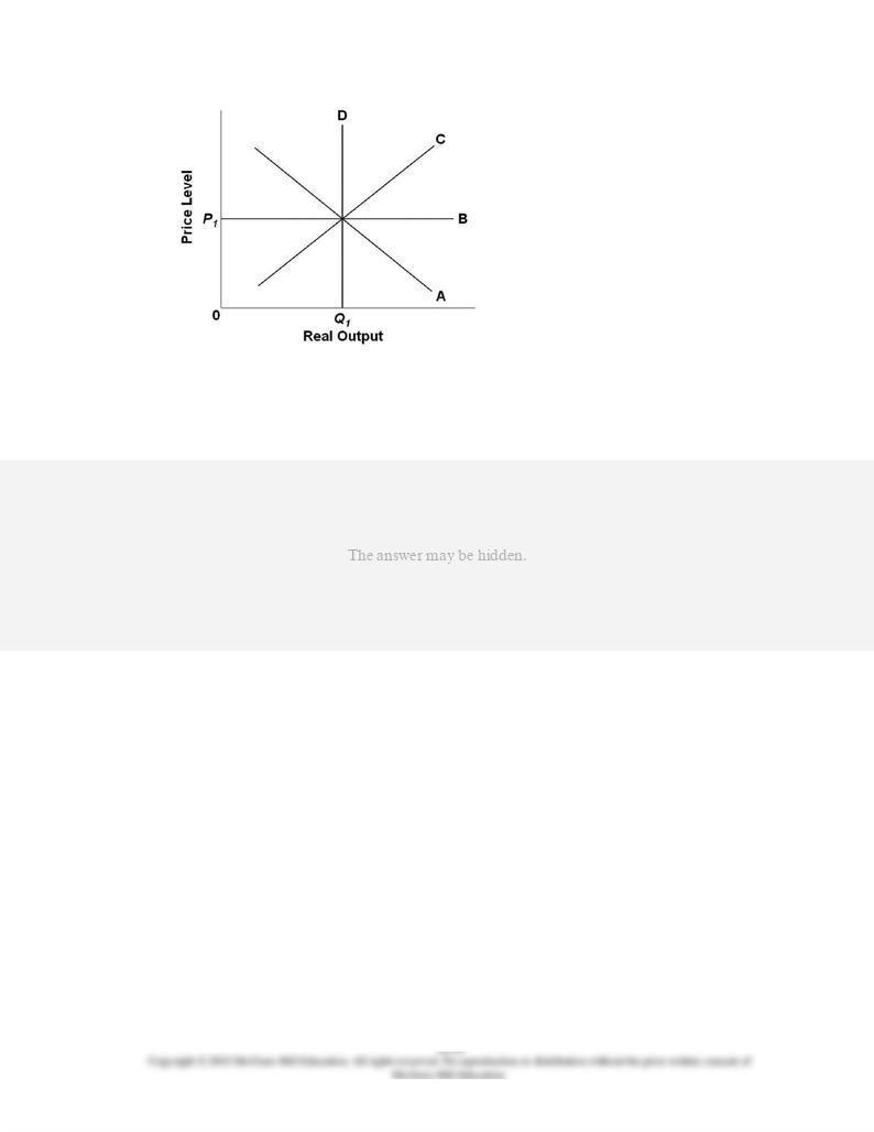
Refer to the diagram. Assume that nominal wages initially are set on the basis of the price
level
P
2 and that the economy initially is operating at its full-employment level of output
Qf
.
In terms of this diagram, the long-run aggregate supply curve:
1,
2, or
3.
AACSB: Reflective Thinking
Blooms: Apply
Difficulty: 2 Medium
Learning Objective: 36-01 Explain the relationship between short-run aggregate supply and long-run aggregate supply.
Topic: From short run to long run
Type: Graph

17.
Refer to the diagram. Assume that nominal wages initially are set on the basis of the price
level
P
2 and that the economy initially is operating at its full-employment level of output
Qf
.
In the short run, demand-pull inflation could best be shown as:
AACSB: Reflective Thinking
Blooms: Analyze
Difficulty: 3 Hard
Learning Objective: 36-01 Explain the relationship between short-run aggregate supply and long-run aggregate supply.
Learning Objective: 36-02 Explain how to apply the "extended" (short-run/long-run) AD-AS model to inflation; recessions;
and economic growth.
Topic: Applying the extended AD-AS model
Topic: From short run to long run
Type: Graph
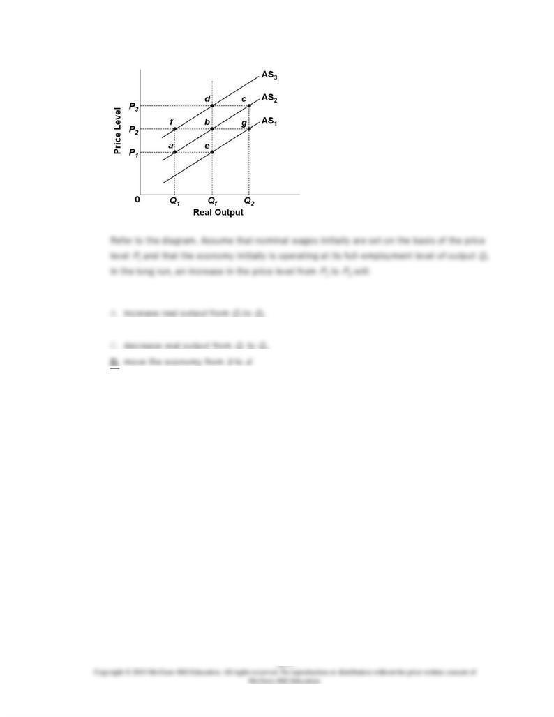
18.
Refer to the diagram. Assume that nominal wages initially are set on the basis of the price
level
P
2 and that the economy initially is operating at its full-employment level of output
Qf
.
In the long run, demand-pull inflation could best be shown as:
AACSB: Reflective Thinking
Blooms: Analyze
Difficulty: 3 Hard
Learning Objective: 36-01 Explain the relationship between short-run aggregate supply and long-run aggregate supply.
Learning Objective: 36-02 Explain how to apply the "extended" (short-run/long-run) AD-AS model to inflation; recessions;
and economic growth.
Topic: Applying the extended AD-AS model
Topic: From short run to long run
Type: Graph
19.
Refer to the diagram. Assume that nominal wages initially are set on the basis of the price
level
P
2 and that the economy initially is operating at its full-employment level of output
Qf
.
In the short run, cost-push inflation could best be shown as:
AACSB: Reflective Thinking
Blooms: Analyze
Difficulty: 3 Hard
Learning Objective: 36-01 Explain the relationship between short-run aggregate supply and long-run aggregate supply.
Learning Objective: 36-02 Explain how to apply the "extended" (short-run/long-run) AD-AS model to inflation; recessions;
and economic growth.
Topic: Applying the extended AD-AS model
Topic: From short run to long run
Type: Graph
20.
Other things equal, the short-run aggregate supply curve shifts positions when:
AACSB: Reflective Thinking
Accessibility: Keyboard Navigation
Blooms: Understand
Difficulty: 2 Medium
Learning Objective: 36-01 Explain the relationship between short-run aggregate supply and long-run aggregate supply.
Topic: From short run to long run
21.
Refer to the diagram relating to short-run and long-run aggregate supply. The:
AACSB: Reflective Thinking
Blooms: Remember
Difficulty: 1 Easy
Learning Objective: 36-01 Explain the relationship between short-run aggregate supply and long-run aggregate supply.
Topic: From short run to long run
Type: Graph
22.
Refer to the diagram. If the price level rises above
P
1 because of an increase in aggregate
demand, the:
1.
AACSB: Reflective Thinking
Blooms: Analyze
Difficulty: 3 Hard
Learning Objective: 36-01 Explain the relationship between short-run aggregate supply and long-run aggregate supply.
Learning Objective: 36-02 Explain how to apply the "extended" (short-run/long-run) AD-AS model to inflation; recessions;
and economic growth.
Topic: Applying the extended AD-AS model
Topic: From short run to long run
Type: Graph
23.
Refer to the diagram. The long-run aggregate supply curve is:
AACSB: Reflective Thinking
Blooms: Remember
Difficulty: 1 Easy
Learning Objective: 36-01 Explain the relationship between short-run aggregate supply and long-run aggregate supply.
Topic: From short run to long run
Type: Graph

24.
Refer to the diagram and assume the economy is operating at equilibrium point
w
. In the
short run, an increase in the price level from
P
2 to
P
3 would move the economy from point
w
to point:
AACSB: Reflective Thinking
Blooms: Analyze
Difficulty: 3 Hard
Learning Objective: 36-01 Explain the relationship between short-run aggregate supply and long-run aggregate supply.
Topic: From short run to long run
Type: Graph

25.
Refer to the diagram and assume the economy is operating at equilibrium point
w
. In the
long run, an increase in the price level from
P
2 to
P
3 would move the economy from point
w
to point:
AACSB: Reflective Thinking
Blooms: Analyze
Difficulty: 3 Hard
Learning Objective: 36-01 Explain the relationship between short-run aggregate supply and long-run aggregate supply.
Topic: From short run to long run
Type: Graph

26.
Refer to the diagram and assume the economy is operating at equilibrium point
w
. In the
short run, a decrease in the price level from
P
2 to
P
1 would move the economy from point
w
to point:
AACSB: Reflective Thinking
Blooms: Analyze
Difficulty: 3 Hard
Learning Objective: 36-01 Explain the relationship between short-run aggregate supply and long-run aggregate supply.
Topic: From short run to long run
Type: Graph

27.
Refer to the diagram and assume the economy is operating at equilibrium point
w
. If
wages and other resource prices are flexible downward, in the long run a decrease in the
price level from
P
2 to
P
1 would move the economy from point
w
to point:
AACSB: Reflective Thinking
Blooms: Analyze
Difficulty: 3 Hard
Learning Objective: 36-01 Explain the relationship between short-run aggregate supply and long-run aggregate supply.
Topic: From short run to long run
Type: Graph
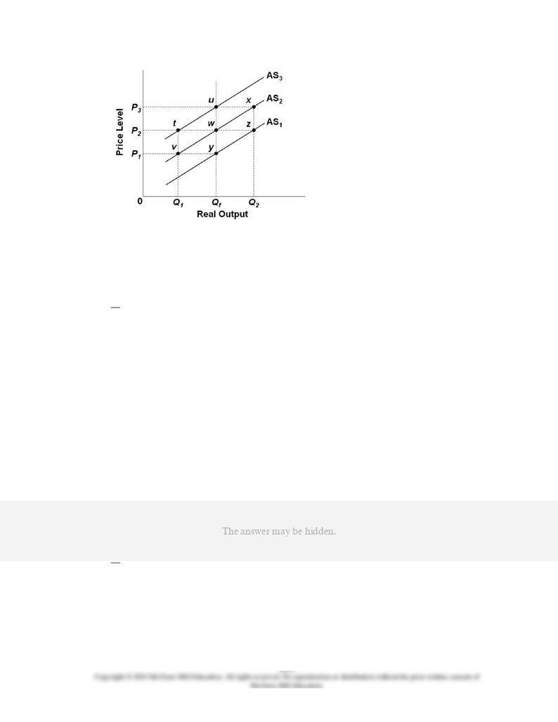
28.
Refer to the diagram. If drawn, the long-run aggregate supply curve would include points:
A.
v
,
w
, and
u
.
B.
y,
w
, and
u
.
C.
t
,
w
, and
z
.
D.
y
,
w
, and
x
.
AACSB: Reflective Thinking
Blooms: Understand
Difficulty: 2 Medium
Learning Objective: 36-01 Explain the relationship between short-run aggregate supply and long-run aggregate supply.
Topic: From short run to long run
Type: Graph
29.
The level of potential output and location of the long-run aggregate supply curve are
determined by:
AACSB: Reflective Thinking
Accessibility: Keyboard Navigation
Blooms: Understand
Difficulty: 2 Medium
Learning Objective: 36-01 Explain the relationship between short-run aggregate supply and long-run aggregate supply.
Topic: From short run to long run

30.
The natural rate of unemployment:
AACSB: Reflective Thinking
Accessibility: Keyboard Navigation
Blooms: Understand
Difficulty: 2 Medium
Learning Objective: 36-01 Explain the relationship between short-run aggregate supply and long-run aggregate supply.
Learning Objective: 36-02 Explain how to apply the "extended" (short-run/long-run) AD-AS model to inflation; recessions;
and economic growth.
Topic: Applying the extended AD-AS model
Topic: From short run to long run
31.
In the extended aggregate demand-aggregate supply model:
AACSB: Reflective Thinking
Accessibility: Keyboard Navigation
Blooms: Understand
Difficulty: 2 Medium
Learning Objective: 36-02 Explain how to apply the "extended" (short-run/long-run) AD-AS model to inflation; recessions;
and economic growth.
Topic: Applying the extended AD-AS model
32.
In the extended aggregate demand-aggregate supply model:
AACSB: Reflective Thinking
Accessibility: Keyboard Navigation
Blooms: Understand
Difficulty: 2 Medium
Learning Objective: 36-02 Explain how to apply the "extended" (short-run/long-run) AD-AS model to inflation; recessions;
and economic growth.
Topic: Applying the extended AD-AS model
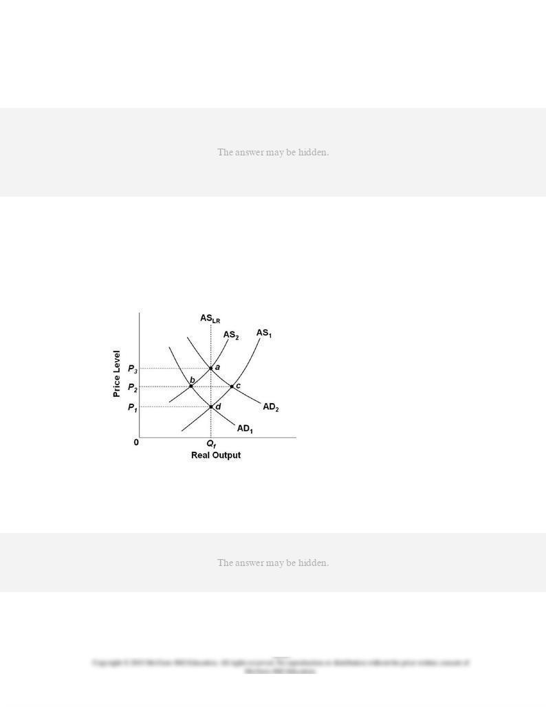
33.
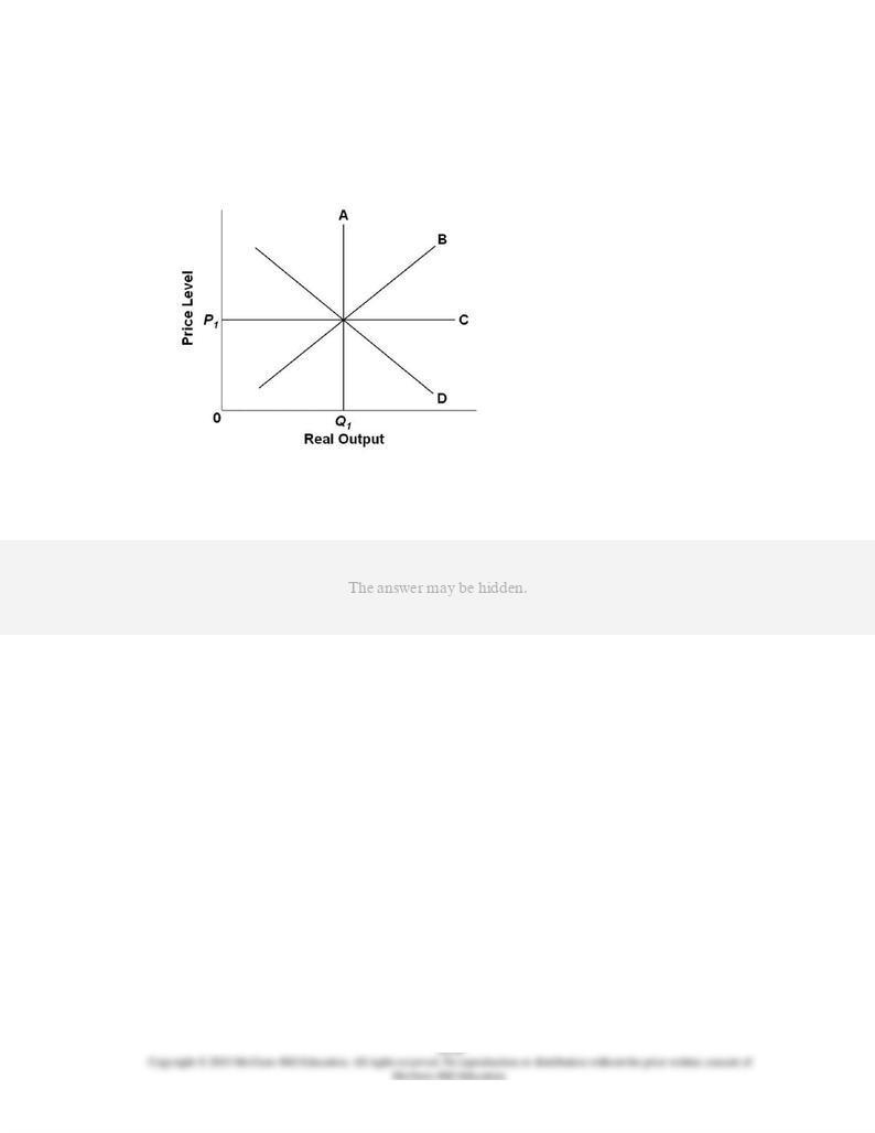
Refer to the diagram. The initial aggregate demand curve is AD1 and the initial aggregate
supply curve is AS1. Demand-pull inflation in the short run is best shown as:
AACSB: Reflective Thinking
Blooms: Apply
Difficulty: 2 Medium
Learning Objective: 36-02 Explain how to apply the "extended" (short-run/long-run) AD-AS model to inflation; recessions;
and economic growth.
Topic: Applying the extended AD-AS model
Type: Graph
34.
Refer to the diagram. The initial aggregate demand curve is AD1 and the initial aggregate
supply curve is AS1. In the long run, demand-pull inflation is best shown as:
AACSB: Reflective Thinking
Blooms: Apply
Difficulty: 2 Medium
Learning Objective: 36-02 Explain how to apply the "extended" (short-run/long-run) AD-AS model to inflation; recessions;
and economic growth.
Topic: Applying the extended AD-AS model
Type: Graph
35.
Refer to the diagram. The initial aggregate demand curve is AD1 and the initial aggregate
supply curve is AS1. In the long run, the aggregate supply curve is vertical in the diagram
because:
AACSB: Reflective Thinking
Blooms: Understand
Difficulty: 2 Medium
Learning Objective: 36-01 Explain the relationship between short-run aggregate supply and long-run aggregate supply.
Learning Objective: 36-02 Explain how to apply the "extended" (short-run/long-run) AD-AS model to inflation; recessions;
and economic growth.
Topic: Applying the extended AD-AS model
Topic: From short run to long run
Type: Graph

36.
Refer to the diagram. The initial aggregate demand curve is AD1 and the initial aggregate
supply curve is AS1. Cost-push inflation in the short run is best represented as a:
AACSB: Reflective Thinking
Blooms: Apply
Difficulty: 2 Medium
Learning Objective: 36-02 Explain how to apply the "extended" (short-run/long-run) AD-AS model to inflation; recessions;
and economic growth.
Topic: Applying the extended AD-AS model
Type: Graph

37.
Refer to the diagram. The initial aggregate demand curve is AD1 and the initial aggregate
supply curve is AS1. Assuming no change in aggregate demand, the long-run response to a
recession caused by cost-push inflation is best depicted as a:
AACSB: Reflective Thinking
Blooms: Apply
Difficulty: 2 Medium
Learning Objective: 36-02 Explain how to apply the "extended" (short-run/long-run) AD-AS model to inflation; recessions;
and economic growth.
Topic: Applying the extended AD-AS model
Type: Graph

38.
1 to
2.
C.
it is possible that aggregate supply will shift rightward from AS2 because nominal wage
2 to
3.
AACSB: Reflective Thinking
Blooms: Analyze
Difficulty: 3 Hard
Learning Objective: 36-02 Explain how to apply the "extended" (short-run/long-run) AD-AS model to inflation; recessions;
and economic growth.
Topic: Applying the extended AD-AS model
Type: Graph
39.
If government uses fiscal policy to restrain cost-push inflation, we can expect:
AACSB: Reflective Thinking
Accessibility: Keyboard Navigation

Blooms: Analyze
Difficulty: 3 Hard
Learning Objective: 36-02 Explain how to apply the "extended" (short-run/long-run) AD-AS model to inflation; recessions;
and economic growth.
Topic: Applying the extended AD-AS model
40.
One policy dilemma posed by cost-push inflation is that:
AACSB: Reflective Thinking
Accessibility: Keyboard Navigation
Blooms: Understand
Difficulty: 2 Medium
Learning Objective: 36-02 Explain how to apply the "extended" (short-run/long-run) AD-AS model to inflation; recessions;
and economic growth.
Topic: Applying the extended AD-AS model
41.
If government uses its stabilization policies to maintain full employment under conditions
of cost-push inflation:
AACSB: Reflective Thinking
Accessibility: Keyboard Navigation
Blooms: Understand
Difficulty: 2 Medium
Learning Objective: 36-02 Explain how to apply the "extended" (short-run/long-run) AD-AS model to inflation; recessions;
and economic growth.
Topic: Applying the extended AD-AS model
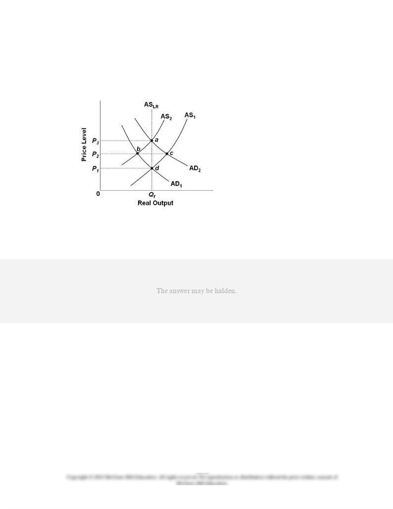
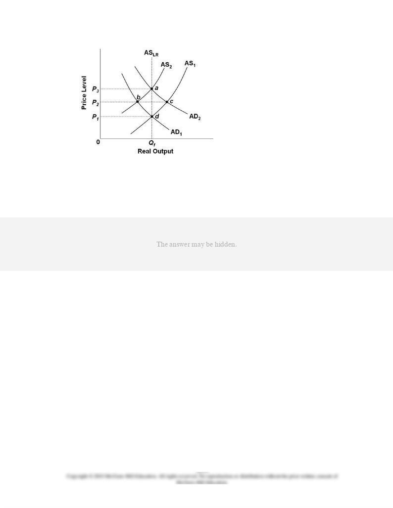
42.
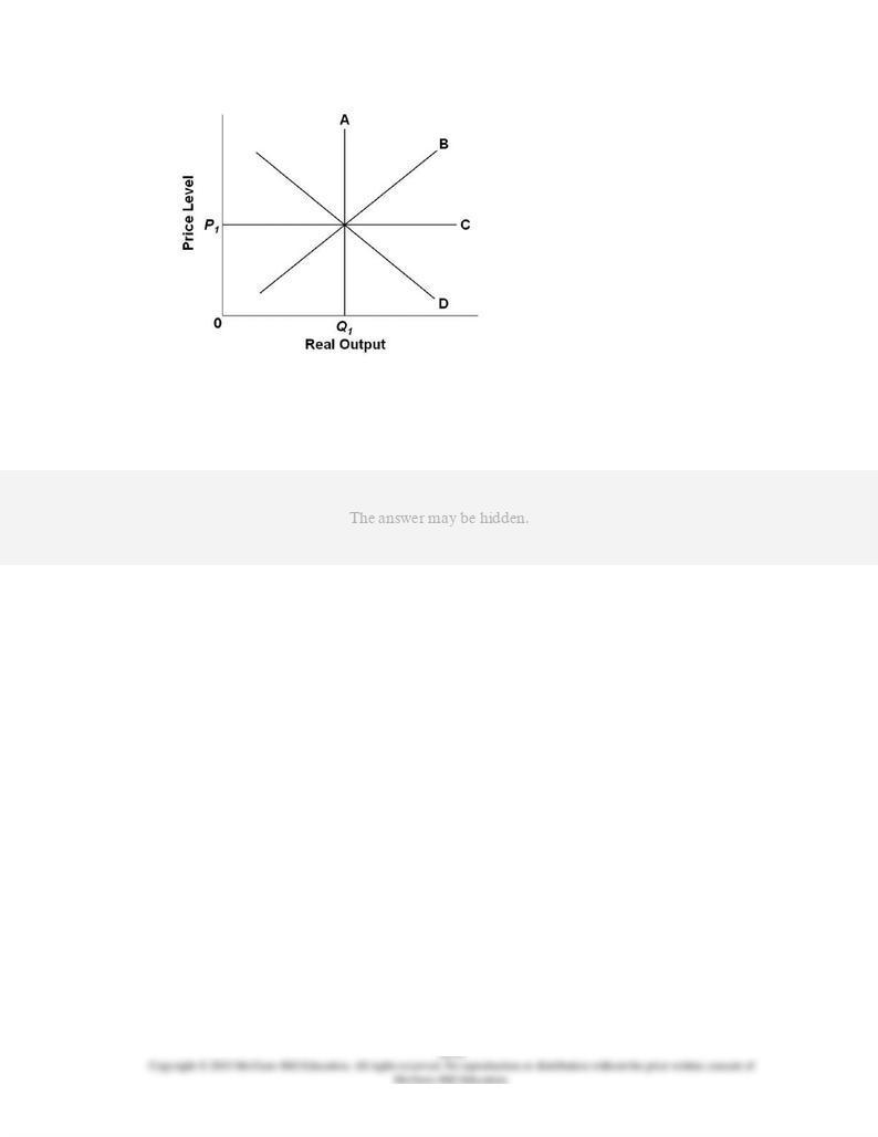
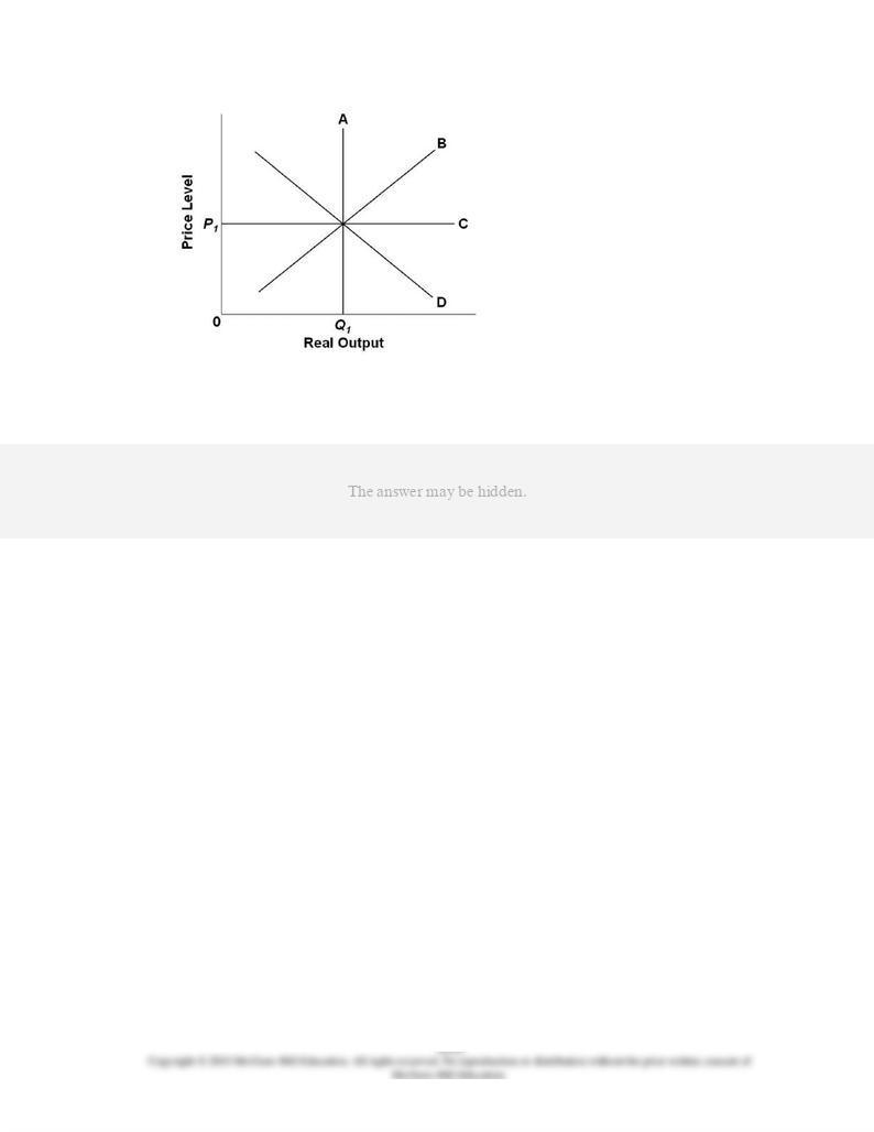
Refer to the diagram and assume that prices and wages are flexible both upward and
downward in the economy. In the extended AD-AS model:
AACSB: Reflective Thinking
Blooms: Analyze
Difficulty: 3 Hard
Learning Objective: 36-02 Explain how to apply the "extended" (short-run/long-run) AD-AS model to inflation; recessions;
and economic growth.
Topic: Applying the extended AD-AS model
Type: Graph

43.
Refer to the diagram and assume that prices and wages are flexible both upward and
downward in the economy. In the extended AD-AS model:
AACSB: Reflective Thinking
Blooms: Analyze
Difficulty: 3 Hard
Learning Objective: 36-02 Explain how to apply the "extended" (short-run/long-run) AD-AS model to inflation; recessions;
and economic growth.
Topic: Applying the extended AD-AS model
Type: Graph

44.
Refer to the diagram and assume that prices and wages are flexible both upward and
downward in the economy. In the extended AD-AS model:
AACSB: Reflective Thinking
Blooms: Analyze
Difficulty: 3 Hard
Learning Objective: 36-02 Explain how to apply the "extended" (short-run/long-run) AD-AS model to inflation; recessions;
and economic growth.
Topic: Applying the extended AD-AS model
Type: Graph

45.
Refer to the diagram and assume that prices and wages are flexible both upward and
downward in the economy. In the extended AD-AS model:
AACSB: Reflective Thinking
Blooms: Analyze
Difficulty: 3 Hard
Learning Objective: 36-02 Explain how to apply the "extended" (short-run/long-run) AD-AS model to inflation; recessions;
and economic growth.
Topic: Applying the extended AD-AS model
Type: Graph

46.
Refer to the diagram. Assume both upward and downward price and wage flexibility in the
economy. In the extended AD-AS model:
AACSB: Reflective Thinking
Blooms: Apply
Difficulty: 2 Medium
Learning Objective: 36-02 Explain how to apply the "extended" (short-run/long-run) AD-AS model to inflation; recessions;
and economic growth.
Topic: Applying the extended AD-AS model
Type: Graph
47.
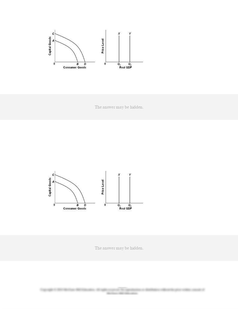
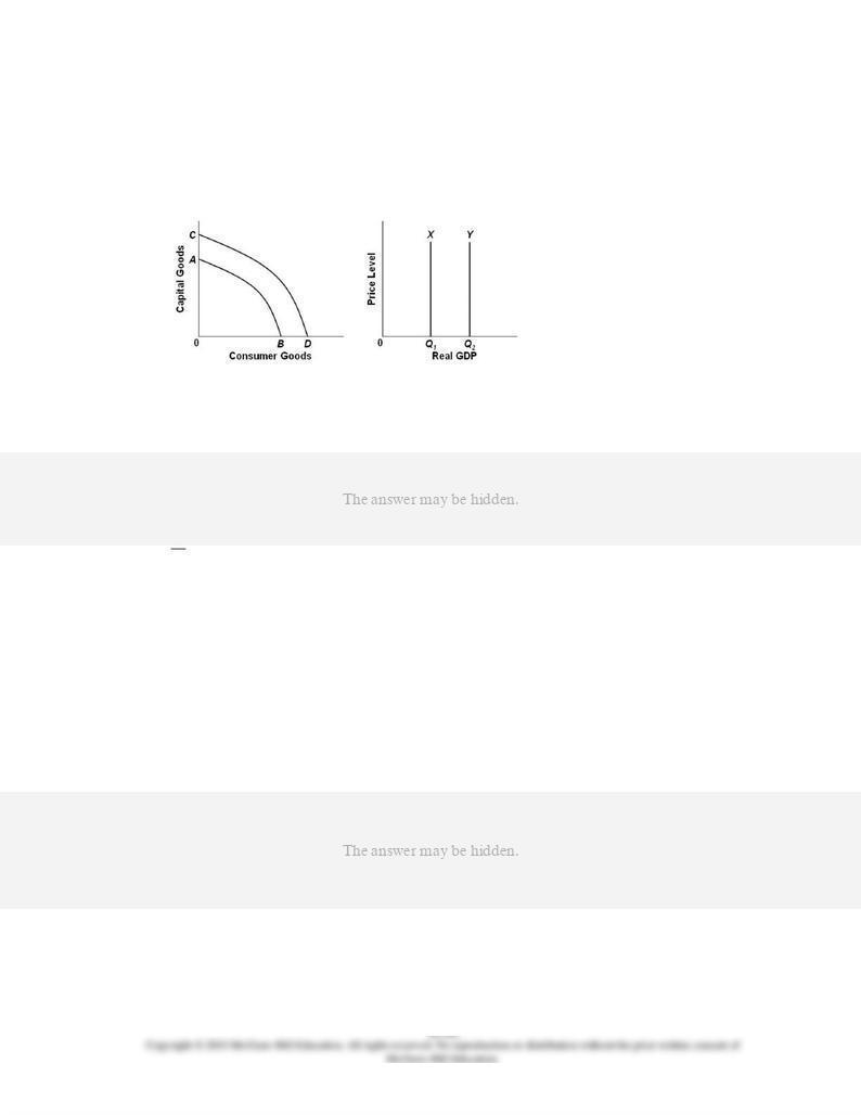
Refer to the graphs. Growth of production capacity is shown by:
AACSB: Reflective Thinking
Blooms: Apply
Difficulty: 2 Medium
Learning Objective: 36-02 Explain how to apply the "extended" (short-run/long-run) AD-AS model to inflation; recessions;
and economic growth.
Topic: Applying the extended AD-AS model
Type: Graph
48.
Refer to the graphs. An increase in an economy's labor productivity would shift curve:
AACSB: Reflective Thinking
Blooms: Analyze
Difficulty: 3 Hard
Learning Objective: 36-02 Explain how to apply the "extended" (short-run/long-run) AD-AS model to inflation; recessions;
and economic growth.
Topic: Applying the extended AD-AS model
Type: Graph
49.
Refer to the graphs. An increase in the economy's human capital would shift curve:
AACSB: Reflective Thinking
Blooms: Analyze
Difficulty: 3 Hard
Learning Objective: 36-02 Explain how to apply the "extended" (short-run/long-run) AD-AS model to inflation; recessions;
and economic growth.
Topic: Applying the extended AD-AS model
Type: Graph
50.
Inflation in the U.S. economy tends to be:
AACSB: Reflective Thinking
Accessibility: Keyboard Navigation
Blooms: Remember
Difficulty: 1 Easy
Learning Objective: 36-02 Explain how to apply the "extended" (short-run/long-run) AD-AS model to inflation; recessions;
and economic growth.
Topic: Applying the extended AD-AS model
51.
In the absence of unexpected shocks, the economy will tend to experience:
AACSB: Reflective Thinking
Accessibility: Keyboard Navigation
Blooms: Remember
Difficulty: 1 Easy
Learning Objective: 36-02 Explain how to apply the "extended" (short-run/long-run) AD-AS model to inflation; recessions;
and economic growth.
Topic: Applying the extended AD-AS model
52.
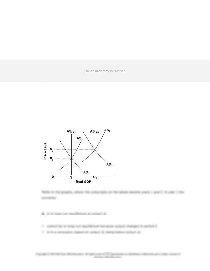
1.
B.
is in short-run equilibrium at output
Q
1, but not in long-run equilibrium.
1 being below output
2.
AACSB: Reflective Thinking
Blooms: Understand
Difficulty: 2 Medium
Learning Objective: 36-02 Explain how to apply the "extended" (short-run/long-run) AD-AS model to inflation; recessions;
and economic growth.
Topic: Applying the extended AD-AS model
Type: Graph
53.
Refer to the graphs, where the subscripts on the labels denote years 1 and 2. From the
graphs we can conclude that from year 1 to year 2:
AACSB: Reflective Thinking
Blooms: Understand
Difficulty: 2 Medium
Learning Objective: 36-02 Explain how to apply the "extended" (short-run/long-run) AD-AS model to inflation; recessions;
and economic growth.
Topic: Applying the extended AD-AS model
Type: Graph
54.
Refer to the graphs, where the subscripts on the labels denote years 1 and 2. From the
graphs we can clearly conclude that the economy:
AACSB: Reflective Thinking
Blooms: Understand
Difficulty: 2 Medium
Learning Objective: 36-02 Explain how to apply the "extended" (short-run/long-run) AD-AS model to inflation; recessions;
and economic growth.
Topic: Applying the extended AD-AS model
Type: Graph
55.
The traditional Phillips Curve suggests a trade-off between:
AACSB: Analytic
Accessibility: Keyboard Navigation
Blooms: Remember
Difficulty: 1 Easy
Learning Objective: 36-03 Explain the short-run trade-off between inflation and unemployment (the Phillips Curve).

Topic: Inflation-unemployment relationship
56.
The basic problem portrayed by the traditional Phillips Curve is:
AACSB: Reflective Thinking
Accessibility: Keyboard Navigation
Blooms: Understand
Difficulty: 2 Medium
Learning Objective: 36-03 Explain the short-run trade-off between inflation and unemployment (the Phillips Curve).
Topic: Inflation-unemployment relationship
57.
The traditional Phillips Curve suggests that, if government uses an expansionary fiscal
policy to stimulate output and employment:
AACSB: Reflective Thinking
Accessibility: Keyboard Navigation
Blooms: Understand
Difficulty: 2 Medium
Learning Objective: 36-03 Explain the short-run trade-off between inflation and unemployment (the Phillips Curve).
Topic: Inflation-unemployment relationship

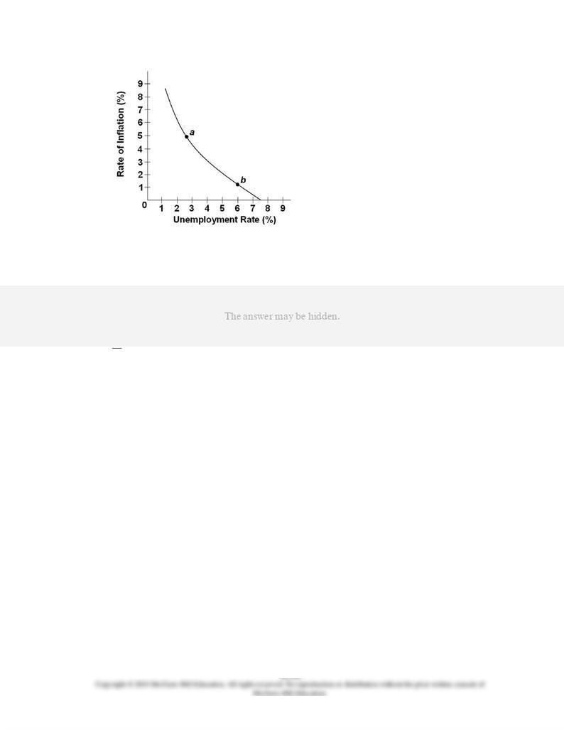
58.
Refer to the diagram for a specific economy. The curve on this graph is known as a:
AACSB: Reflective Thinking
Blooms: Remember
Difficulty: 1 Easy
Learning Objective: 36-03 Explain the short-run trade-off between inflation and unemployment (the Phillips Curve).
Topic: Inflation-unemployment relationship
Type: Graph
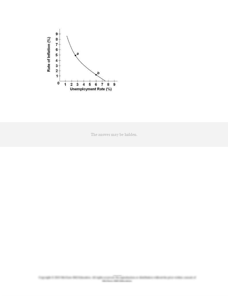
59.
Refer to the diagram for a specific economy. Which of the following best describes the
relationship shown by this curve?
AACSB: Reflective Thinking
Blooms: Understand
Difficulty: 2 Medium
Learning Objective: 36-03 Explain the short-run trade-off between inflation and unemployment (the Phillips Curve).
Topic: Inflation-unemployment relationship
Type: Graph

60.
Refer to the diagram for a specific economy. A reduction in structural unemployment or
bottleneck problems in labor markets will:
AACSB: Reflective Thinking
Blooms: Analyze
Difficulty: 3 Hard
Learning Objective: 36-03 Explain the short-run trade-off between inflation and unemployment (the Phillips Curve).
Topic: Inflation-unemployment relationship
Type: Graph
61.
Refer to the diagram for a specific economy. An increase in aggregate demand will:
AACSB: Reflective Thinking
Blooms: Analyze
Difficulty: 3 Hard
Learning Objective: 36-03 Explain the short-run trade-off between inflation and unemployment (the Phillips Curve).
Topic: Inflation-unemployment relationship
Type: Graph
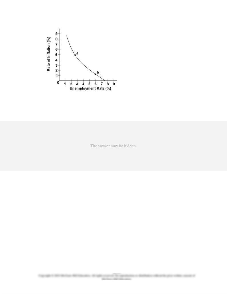
62.
Refer to the diagram for a specific economy. Which of the following best describes a
decision by policymakers that moves this economy from point
b
to point
a
?
AACSB: Reflective Thinking
Blooms: Apply
Difficulty: 2 Medium
Learning Objective: 36-03 Explain the short-run trade-off between inflation and unemployment (the Phillips Curve).
Topic: Inflation-unemployment relationship
Type: Graph
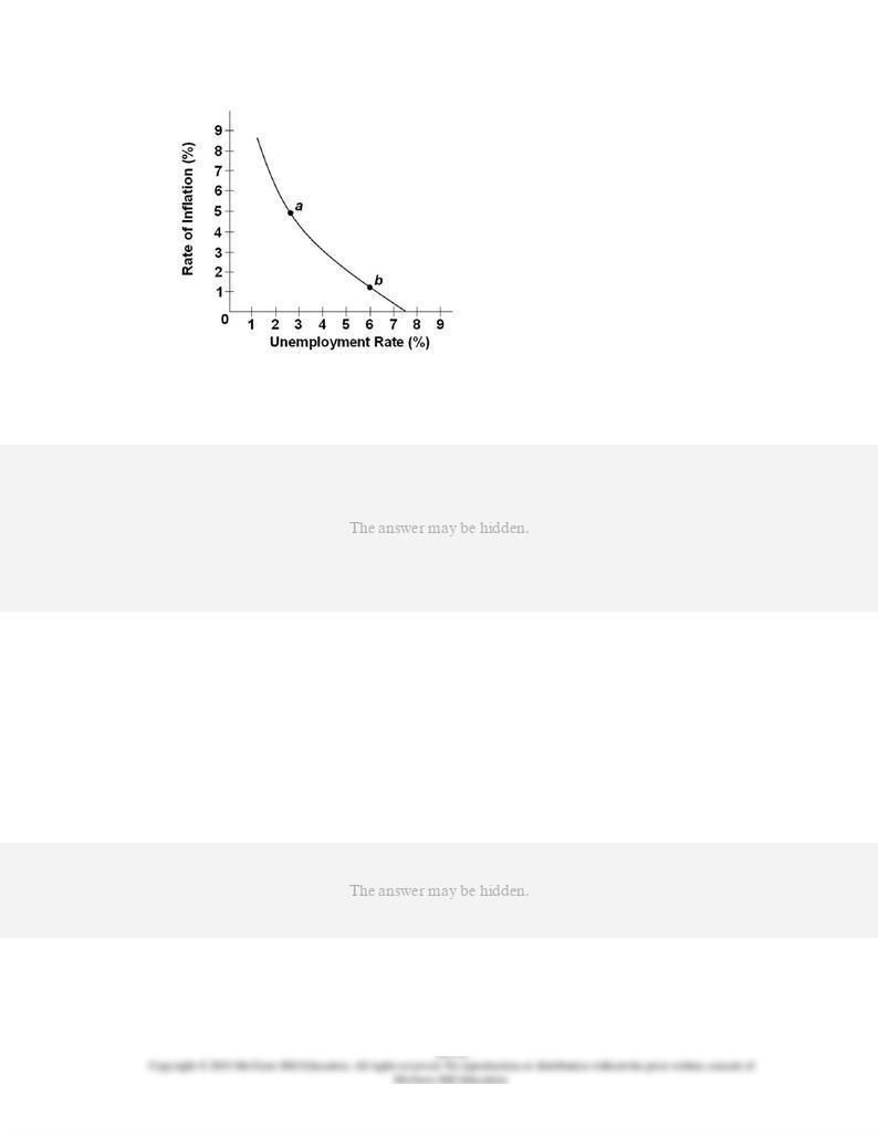
63.
Refer to the diagram for a specific economy. The shape of this curve suggests that:
AACSB: Reflective Thinking
Blooms: Understand
Difficulty: 2 Medium
Learning Objective: 36-03 Explain the short-run trade-off between inflation and unemployment (the Phillips Curve).
Topic: Inflation-unemployment relationship
Type: Graph
64.
Stagflation refers to:
AACSB: Analytic
Accessibility: Keyboard Navigation
Blooms: Remember

Difficulty: 1 Easy
Learning Objective: 36-03 Explain the short-run trade-off between inflation and unemployment (the Phillips Curve).
Topic: Inflation-unemployment relationship
65.
Inflation accompanied by falling real output and employment is known as:
AACSB: Analytic
Accessibility: Keyboard Navigation
Blooms: Remember
Difficulty: 1 Easy
Learning Objective: 36-03 Explain the short-run trade-off between inflation and unemployment (the Phillips Curve).
Topic: Inflation-unemployment relationship
66.
Which of the following allegedly contributed to the stagflation in the mid-1970s?
AACSB: Reflective Thinking
Accessibility: Keyboard Navigation
Blooms: Remember
Difficulty: 1 Easy
Learning Objective: 36-03 Explain the short-run trade-off between inflation and unemployment (the Phillips Curve).
Topic: Inflation-unemployment relationship

67.
Statistical data for the 1970s and 1980s suggest that:
AACSB: Reflective Thinking
Accessibility: Keyboard Navigation
Blooms: Remember
Difficulty: 1 Easy
Learning Objective: 36-03 Explain the short-run trade-off between inflation and unemployment (the Phillips Curve).
Topic: Inflation-unemployment relationship
68.
A rightward shift of the traditional Phillips Curve would suggest that:
AACSB: Reflective Thinking
Accessibility: Keyboard Navigation
Blooms: Understand
Difficulty: 2 Medium
Learning Objective: 36-03 Explain the short-run trade-off between inflation and unemployment (the Phillips Curve).
Topic: Inflation-unemployment relationship
69.
Rightward and upward shifts of the Phillips Curve in the 1970s and early 1980s were
caused by:
AACSB: Reflective Thinking
Accessibility: Keyboard Navigation
Blooms: Remember

Difficulty: 1 Easy
Learning Objective: 36-03 Explain the short-run trade-off between inflation and unemployment (the Phillips Curve).
Topic: Inflation-unemployment relationship
70.
An adverse aggregate supply shock could result from:
AACSB: Reflective Thinking
Accessibility: Keyboard Navigation
Blooms: Apply
Difficulty: 2 Medium
Learning Objective: 36-03 Explain the short-run trade-off between inflation and unemployment (the Phillips Curve).
Topic: Inflation-unemployment relationship
71.
An adverse aggregate supply shock:
AACSB: Reflective Thinking
Accessibility: Keyboard Navigation
Blooms: Understand
Difficulty: 2 Medium
Learning Objective: 36-03 Explain the short-run trade-off between inflation and unemployment (the Phillips Curve).
Topic: Inflation-unemployment relationship

72.
The last few years of the 1990s in the United States were characterized by:
AACSB: Reflective Thinking
Accessibility: Keyboard Navigation
Blooms: Remember
Difficulty: 1 Easy
Learning Objective: 36-03 Explain the short-run trade-off between inflation and unemployment (the Phillips Curve).
Topic: Inflation-unemployment relationship
73.
Which of the following is a true statement?
AACSB: Reflective Thinking
Accessibility: Keyboard Navigation
Blooms: Understand
Difficulty: 2 Medium
Learning Objective: 36-04 Discuss why there is no long-run trade-off between inflation and unemployment.
Topic: Long-run Phillips Curve
74.
Which of the following is a true statement?
AACSB: Reflective Thinking
Accessibility: Keyboard Navigation
Blooms: Remember

Difficulty: 1 Easy
Learning Objective: 36-04 Discuss why there is no long-run trade-off between inflation and unemployment.
Topic: Long-run Phillips Curve
75.
Which of the following is a true statement?
AACSB: Reflective Thinking
Accessibility: Keyboard Navigation
Blooms: Remember
Difficulty: 1 Easy
Learning Objective: 36-04 Discuss why there is no long-run trade-off between inflation and unemployment.
Topic: Long-run Phillips Curve
76.
In the last half of the 1990s, the usual short-run trade-off between inflation and
unemployment did not arise because:
AACSB: Reflective Thinking
Accessibility: Keyboard Navigation
Blooms: Remember
Difficulty: 1 Easy
Learning Objective: 36-04 Discuss why there is no long-run trade-off between inflation and unemployment.
Topic: Long-run Phillips Curve

77.
Suppose that the Consumer Price Index for a particular economy rose from 110 to 120 in
year 1, 120 to 130 in year 2, and 130 to 140 in year 3. We could conclude that this economy
is experiencing:
AACSB: Analytic
Accessibility: Keyboard Navigation
Blooms: Apply
Difficulty: 2 Medium
Learning Objective: 36-04 Discuss why there is no long-run trade-off between inflation and unemployment.
Topic: Long-run Phillips Curve
78.
Disinflation occurs when:
AACSB: Analytic
Accessibility: Keyboard Navigation
Blooms: Remember
Difficulty: 1 Easy
Learning Objective: 36-04 Discuss why there is no long-run trade-off between inflation and unemployment.
Topic: Long-run Phillips Curve

79.
As distinct from reductions in the price level, reductions in the rate of inflation are referred
to as:
AACSB: Analytic
Accessibility: Keyboard Navigation
Blooms: Remember
Difficulty: 1 Easy
Learning Objective: 36-04 Discuss why there is no long-run trade-off between inflation and unemployment.
Topic: Long-run Phillips Curve
80.
When the actual rate of inflation is less than the expected rate:
AACSB: Reflective Thinking
Accessibility: Keyboard Navigation
Blooms: Understand
Difficulty: 2 Medium
Learning Objective: 36-04 Discuss why there is no long-run trade-off between inflation and unemployment.
Topic: Long-run Phillips Curve
81.
When the actual rate of inflation exceeds the expected rate:
AACSB: Reflective Thinking
Accessibility: Keyboard Navigation
Blooms: Understand
Difficulty: 2 Medium
Learning Objective: 36-04 Discuss why there is no long-run trade-off between inflation and unemployment.
Topic: Long-run Phillips Curve
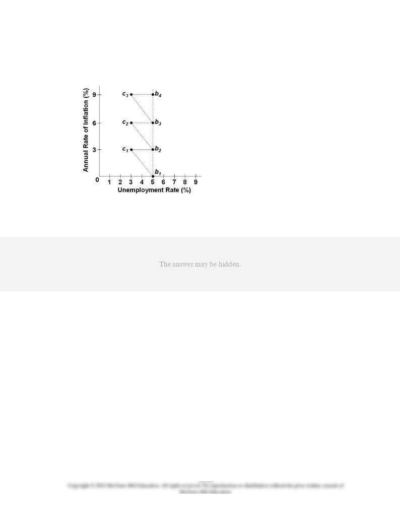
82.
The diagram is the basis for explaining:
AACSB: Reflective Thinking
Blooms: Apply
Difficulty: 2 Medium
Learning Objective: 36-04 Discuss why there is no long-run trade-off between inflation and unemployment.
Topic: Long-run Phillips Curve
Type: Graph
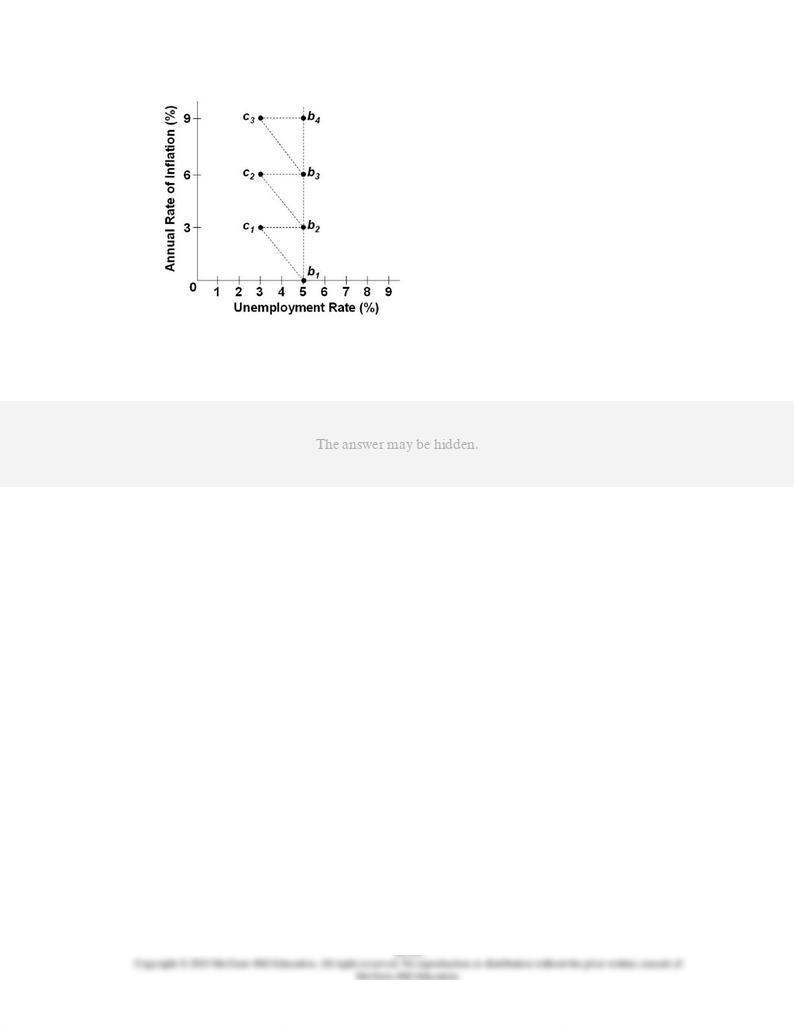
83.
Refer to the diagram. The natural rate of unemployment for this economy is:
AACSB: Analytic
Blooms: Apply
Difficulty: 2 Medium
Learning Objective: 36-04 Discuss why there is no long-run trade-off between inflation and unemployment.
Topic: Long-run Phillips Curve
Type: Graph
84.
1. With a time lag between
price and nominal wage adjustments, an increase in aggregate demand will temporarily
2 to
1.
1 to
2.
1 to
1.
1 to
2.
AACSB: Reflective Thinking
Blooms: Analyze
Difficulty: 3 Hard
Learning Objective: 36-04 Discuss why there is no long-run trade-off between inflation and unemployment.
Topic: Long-run Phillips Curve
Type: Graph
85.
1. Which of the
following movements is consistent with the traditional Phillips Curve?
1 to
2.
1 to
1.
1 to
2.
2 to
1.
AACSB: Reflective Thinking
Blooms: Understand
Difficulty: 2 Medium
Learning Objective: 36-04 Discuss why there is no long-run trade-off between inflation and unemployment.
Topic: Long-run Phillips Curve
Type: Graph
86.
1. Point
1 represents:
AACSB: Reflective Thinking
Blooms: Understand
Difficulty: 2 Medium
Learning Objective: 36-04 Discuss why there is no long-run trade-off between inflation and unemployment.
Topic: Long-run Phillips Curve
Type: Graph
87.
1. The long-run
relationship between the unemployment rate and the rate of inflation is represented by:
1 and
1.
1,
2,
3, and
4.
1 and
2.
AACSB: Reflective Thinking
Blooms: Apply
Difficulty: 2 Medium
Learning Objective: 36-04 Discuss why there is no long-run trade-off between inflation and unemployment.
Topic: Long-run Phillips Curve
Type: Graph
88.
Government can push the unemployment rate below the natural rate only by:
AACSB: Reflective Thinking
Accessibility: Keyboard Navigation
Blooms: Understand
Difficulty: 2 Medium
Learning Objective: 36-04 Discuss why there is no long-run trade-off between inflation and unemployment.
Topic: Long-run Phillips Curve

89.
In the long run:
AACSB: Reflective Thinking
Accessibility: Keyboard Navigation
Blooms: Understand
Difficulty: 2 Medium
Learning Objective: 36-04 Discuss why there is no long-run trade-off between inflation and unemployment.
Topic: Long-run Phillips Curve

90.
Refer to the diagram. Assume that the natural rate of unemployment is 5 percent and that
the economy is initially operating at point
a
, where the expected and actual rates of
inflation are each 6 percent. If the actual rate of inflation unexpectedly falls from 6 percent
to 4 percent, then the unemployment rate will:
AACSB: Analytic
Blooms: Analyze
Difficulty: 3 Hard
Learning Objective: 36-04 Discuss why there is no long-run trade-off between inflation and unemployment.
Topic: Long-run Phillips Curve
Type: Graph
91.
Refer to the diagram. Assume that the natural rate of unemployment is 5 percent and that
the economy is initially operating at point
a
, where the expected and actual rates of
inflation are each 6 percent. In the long run, the decline in the actual rate of inflation from
6 percent to 4 percent will:
AACSB: Reflective Thinking
Blooms: Analyze
Difficulty: 3 Hard
Learning Objective: 36-04 Discuss why there is no long-run trade-off between inflation and unemployment.
Topic: Long-run Phillips Curve
Type: Graph

92.
Refer to the diagram. Assume that the natural rate of unemployment is 5 percent and that
the economy is initially operating at point
c
, where the expected and actual rates of
inflation are each 4 percent. If the actual rate of inflation unexpectedly rises from 4
percent to 6 percent, the economy will:
AACSB: Reflective Thinking
Blooms: Analyze
Difficulty: 3 Hard
Learning Objective: 36-04 Discuss why there is no long-run trade-off between inflation and unemployment.
Topic: Long-run Phillips Curve
Type: Graph
93.
In the diagram:
AACSB: Reflective Thinking
Blooms: Understand
Difficulty: 2 Medium
Learning Objective: 36-04 Discuss why there is no long-run trade-off between inflation and unemployment.
Topic: Long-run Phillips Curve
Type: Graph
94.
Refer to the diagram. Point
b
on short-run Phillips Curve PC1 represents a rate of:
AACSB: Reflective Thinking
Blooms: Understand
Difficulty: 2 Medium
Learning Objective: 36-04 Discuss why there is no long-run trade-off between inflation and unemployment.
Topic: Long-run Phillips Curve
Type: Graph
95.
Refer to the diagram. Point
b
would be explained by:
AACSB: Reflective Thinking
Blooms: Understand
Difficulty: 2 Medium
Learning Objective: 36-04 Discuss why there is no long-run trade-off between inflation and unemployment.
Topic: Long-run Phillips Curve
Type: Graph

96.
Refer to the diagram. Point
b
would not be permanent because the:
AACSB: Reflective Thinking
Blooms: Analyze
Difficulty: 3 Hard
Learning Objective: 36-04 Discuss why there is no long-run trade-off between inflation and unemployment.
Topic: Long-run Phillips Curve
Type: Graph
97.
Refer to the diagram. The move of the economy from
c
to
e
on short-run Phillips Curve PC2
would be explained by an:
AACSB: Reflective Thinking
Blooms: Understand
Difficulty: 2 Medium
Learning Objective: 36-04 Discuss why there is no long-run trade-off between inflation and unemployment.
Topic: Long-run Phillips Curve
Type: Graph
98.
Which of the following is a tenet of supply-side economics?
AACSB: Reflective Thinking
Accessibility: Keyboard Navigation
Blooms: Remember
Difficulty: 1 Easy
Learning Objective: 36-05 Explain the relationship between tax rates; tax revenues; and aggregate supply.
Topic: Taxation and aggregate supply
99.
The Laffer Curve is a central concept in:
AACSB: Reflective Thinking
Accessibility: Keyboard Navigation
Blooms: Remember
Difficulty: 1 Easy
Learning Objective: 36-05 Explain the relationship between tax rates; tax revenues; and aggregate supply.
Topic: Taxation and aggregate supply
100.
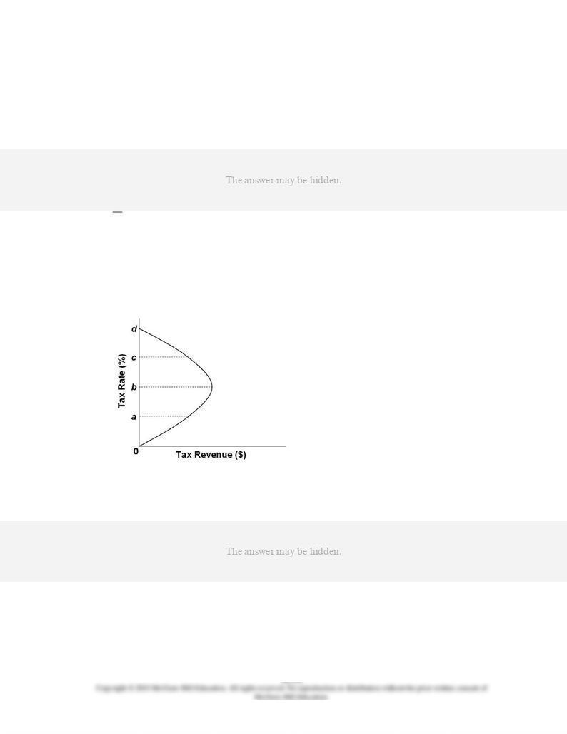
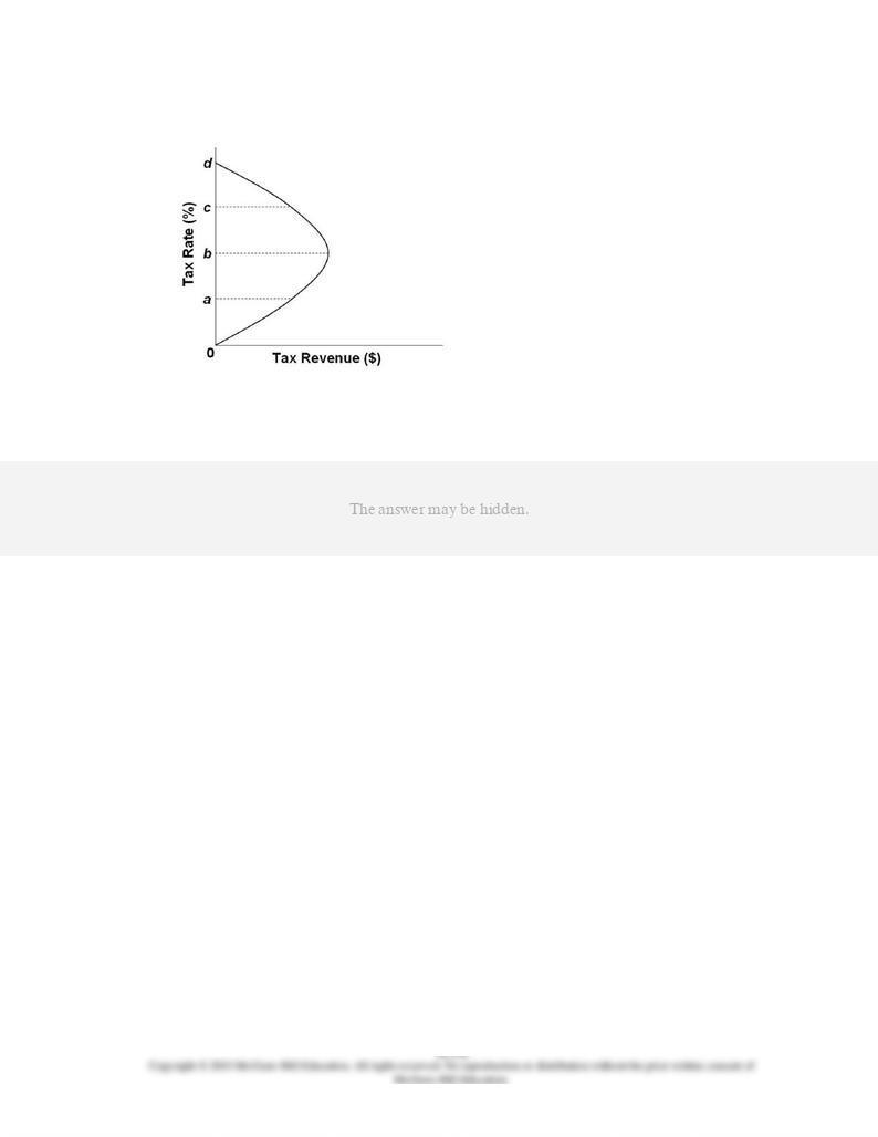
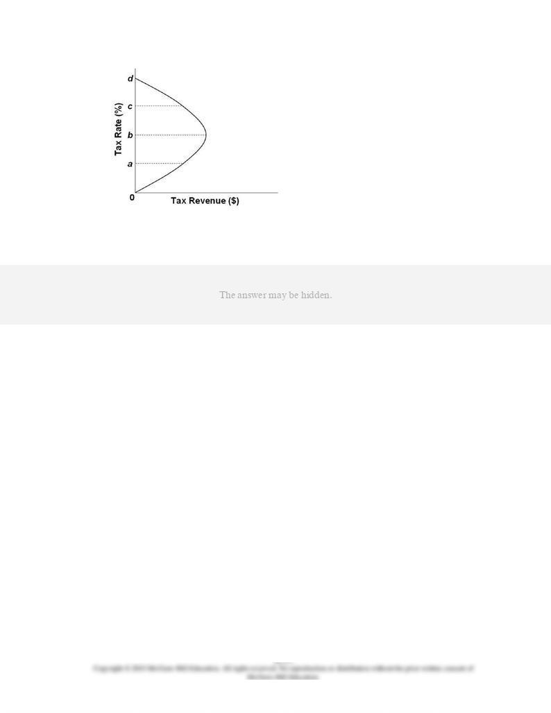
The given curve is known as the:
AACSB: Reflective Thinking
Blooms: Remember
Difficulty: 1 Easy
Learning Objective: 36-05 Explain the relationship between tax rates; tax revenues; and aggregate supply.
Topic: Taxation and aggregate supply
Type: Graph
101.
Refer to the diagram. Supply-side economists believe that tax rates are typically:
AACSB: Reflective Thinking
Blooms: Understand
Difficulty: 2 Medium
Learning Objective: 36-05 Explain the relationship between tax rates; tax revenues; and aggregate supply.
Topic: Taxation and aggregate supply
Type: Graph
102.
In the curve, a decline in the tax rate from
c
to
b
would:
AACSB: Reflective Thinking
Blooms: Analyze
Difficulty: 3 Hard
Learning Objective: 36-05 Explain the relationship between tax rates; tax revenues; and aggregate supply.
Topic: Taxation and aggregate supply
Type: Graph
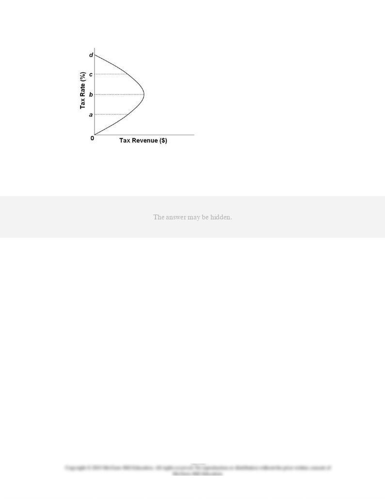
103.
Refer to the diagram. If the tax rate is currently
c
and the government wants to maximize
tax revenue, it should:
AACSB: Reflective Thinking
Blooms: Analyze
Difficulty: 3 Hard
Learning Objective: 36-05 Explain the relationship between tax rates; tax revenues; and aggregate supply.
Topic: Taxation and aggregate supply
Type: Graph
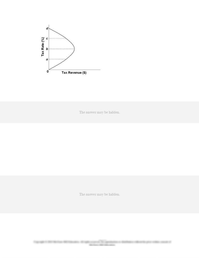
104.
Refer to the diagram. The general agreement of most economists is that the U.S. economy
today is:
AACSB: Reflective Thinking
Blooms: Understand
Difficulty: 2 Medium
Learning Objective: 36-05 Explain the relationship between tax rates; tax revenues; and aggregate supply.
Topic: Taxation and aggregate supply
Type: Graph
105.
Supply-side economist Arthur Laffer has argued that:
AACSB: Reflective Thinking
Accessibility: Keyboard Navigation
Blooms: Remember

Difficulty: 1 Easy
Learning Objective: 36-05 Explain the relationship between tax rates; tax revenues; and aggregate supply.
Topic: Taxation and aggregate supply
106.
A basic criticism of supply-side economics is that:
AACSB: Reflective Thinking
Accessibility: Keyboard Navigation
Blooms: Remember
Difficulty: 1 Easy
Learning Objective: 36-05 Explain the relationship between tax rates; tax revenues; and aggregate supply.
Topic: Taxation and aggregate supply
107.
Critics of supply-side economics:
AACSB: Reflective Thinking
Accessibility: Keyboard Navigation
Blooms: Remember
Difficulty: 1 Easy
Learning Objective: 36-05 Explain the relationship between tax rates; tax revenues; and aggregate supply.
Topic: Taxation and aggregate supply
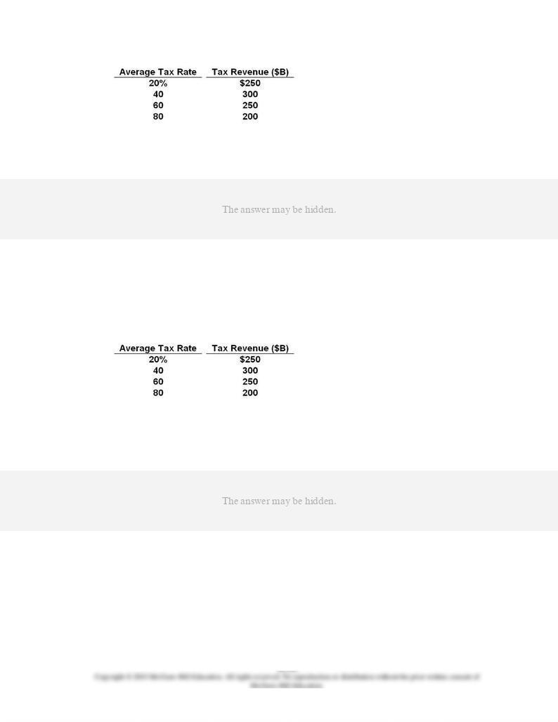
108.
If graphed, the relationship shown would depict this economy's:
AACSB: Analytic
Blooms: Apply
Difficulty: 2 Medium
Learning Objective: 36-05 Explain the relationship between tax rates; tax revenues; and aggregate supply.
Topic: Taxation and aggregate supply
Type: Table
109.
Refer to the table. If the current tax rate is 60 percent, supply-side economists would
advocate:
AACSB: Analytic
Blooms: Apply
Difficulty: 2 Medium
Learning Objective: 36-05 Explain the relationship between tax rates; tax revenues; and aggregate supply.
Topic: Taxation and aggregate supply
Type: Table

110.
In 1993 the federal government boosted income tax rates. In the seven years that
followed:
AACSB: Reflective Thinking
Accessibility: Keyboard Navigation
Blooms: Remember
Difficulty: 1 Easy
Learning Objective: 36-05 Explain the relationship between tax rates; tax revenues; and aggregate supply.
Topic: Taxation and aggregate supply
111.
In 1993 the federal government boosted income tax rates. The change in tax revenue that
occurred in the seven years that followed:
AACSB: Reflective Thinking
Accessibility: Keyboard Navigation
Blooms: Apply
Difficulty: 2 Medium
Learning Objective: 36-05 Explain the relationship between tax rates; tax revenues; and aggregate supply.
Topic: Taxation and aggregate supply

112.
(Consider This) The ideas of economist Arthur Laffer became the centerpiece for tax
policy during the:
AACSB: Reflective Thinking
Accessibility: Keyboard Navigation
Blooms: Remember
Difficulty: 1 Easy
Learning Objective: 36-05 Explain the relationship between tax rates; tax revenues; and aggregate supply.
Topic: Taxation and aggregate supply
113.
(Consider This) Economist Arthur Laffer equated Robin Hood to:
AACSB: Reflective Thinking
Accessibility: Keyboard Navigation
Blooms: Remember
Difficulty: 1 Easy
Learning Objective: 36-05 Explain the relationship between tax rates; tax revenues; and aggregate supply.
Topic: Taxation and aggregate supply

114.
(Last Word) According to the research of Christina Romer and David Romer:
AACSB: Reflective Thinking
Accessibility: Keyboard Navigation
Blooms: Remember
Difficulty: 1 Easy
Learning Objective: 36-05 Explain the relationship between tax rates; tax revenues; and aggregate supply.
Topic: Taxation and aggregate supply
115.
(Last Word) According to the research of Christina Romer and David Romer, tax increases
implemented to reduce an inherited budget deficit:
AACSB: Reflective Thinking
Accessibility: Keyboard Navigation
Blooms: Remember
Difficulty: 1 Easy
Learning Objective: 36-05 Explain the relationship between tax rates; tax revenues; and aggregate supply.
Topic: Taxation and aggregate supply
True / False Questions

116.
The short-run aggregate supply curve is vertical and the long-run aggregate supply curve
is horizontal.
AACSB: Reflective Thinking
Accessibility: Keyboard Navigation
Blooms: Remember
Difficulty: 1 Easy
Learning Objective: 36-01 Explain the relationship between short-run aggregate supply and long-run aggregate supply.
Topic: From short run to long run
117.
The short-run aggregate supply curve shifts to the left when nominal wages rise in
response to price level increases.
AACSB: Reflective Thinking
Accessibility: Keyboard Navigation
Blooms: Understand
Difficulty: 2 Medium
Learning Objective: 36-01 Explain the relationship between short-run aggregate supply and long-run aggregate supply.
Topic: From short run to long run
118.
In the extended AD-AS model, the long-run aggregate supply curve is vertical.
AACSB: Reflective Thinking
Accessibility: Keyboard Navigation
Blooms: Remember
Difficulty: 1 Easy
Learning Objective: 36-01 Explain the relationship between short-run aggregate supply and long-run aggregate supply.
Learning Objective: 36-02 Explain how to apply the "extended" (short-run/long-run) AD-AS model to inflation; recessions;
and economic growth.
Topic: Applying the extended AD-AS model
Topic: From short run to long run

119.
Demand-pull inflation and cost-push inflation are identical concepts because both involve
lower unemployment rates and rising prices.
AACSB: Reflective Thinking
Accessibility: Keyboard Navigation
Blooms: Understand
Difficulty: 2 Medium
Learning Objective: 36-02 Explain how to apply the "extended" (short-run/long-run) AD-AS model to inflation; recessions;
and economic growth.
Topic: Applying the extended AD-AS model
120.
The Phillips Curve suggests an inverse relationship between increases in the price level
and the level of employment.
AACSB: Reflective Thinking
Accessibility: Keyboard Navigation
Blooms: Understand
Difficulty: 2 Medium
Learning Objective: 36-03 Explain the short-run trade-off between inflation and unemployment (the Phillips Curve).
Topic: Inflation-unemployment relationship
121.
A shift in the Phillips Curve to the left will improve the short-run inflation-unemployment
choices available to society.
AACSB: Reflective Thinking
Accessibility: Keyboard Navigation
Blooms: Understand
Difficulty: 2 Medium
Learning Objective: 36-03 Explain the short-run trade-off between inflation and unemployment (the Phillips Curve).
Topic: Inflation-unemployment relationship
122.
A rightward and upward shift of the Phillips Curve is consistent with the occurrence of
stagflation.
AACSB: Reflective Thinking

Accessibility: Keyboard Navigation
Blooms: Understand
Difficulty: 2 Medium
Learning Objective: 36-03 Explain the short-run trade-off between inflation and unemployment (the Phillips Curve).
Topic: Inflation-unemployment relationship
123.
There is no trade-off between unemployment and inflation in the long run.
AACSB: Reflective Thinking
Accessibility: Keyboard Navigation
Blooms: Understand
Difficulty: 2 Medium
Learning Objective: 36-04 Discuss why there is no long-run trade-off between inflation and unemployment.
Topic: Long-run Phillips Curve
124.
The Laffer Curve shows the trade-off between the price level and tax rates.
AACSB: Analytic
Accessibility: Keyboard Navigation
Blooms: Remember
Difficulty: 1 Easy
Learning Objective: 36-05 Explain the relationship between tax rates; tax revenues; and aggregate supply.
Topic: Taxation and aggregate supply
125.
The Laffer Curve underlies the contention that lower tax rates need not reduce tax
revenues.
AACSB: Reflective Thinking
Accessibility: Keyboard Navigation
Blooms: Understand
Difficulty: 2 Medium
Learning Objective: 36-05 Explain the relationship between tax rates; tax revenues; and aggregate supply.
Topic: Taxation and aggregate supply
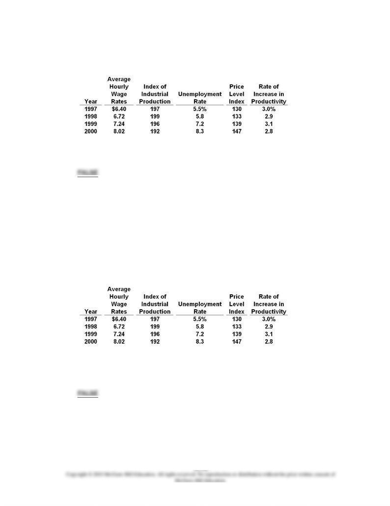
126.
Answer the question on the basis of the following economic data for a hypothetical
economy:
The given data indicate that the economy has entered a period of demand-pull inflation.
AACSB: Analytic
Blooms: Apply
Difficulty: 2 Medium
Learning Objective: 36-02 Explain how to apply the "extended" (short-run/long-run) AD-AS model to inflation; recessions;
and economic growth.
Topic: Applying the extended AD-AS model
Type: Table
127.
Answer the question on the basis of the following economic data for a hypothetical
economy:
Refer to the given data. It would be the appropriate stabilization policy to raise interest
rates, raise taxes, and reduce government expenditures.
AACSB: Reflective Thinking
Blooms: Analyze
Difficulty: 3 Hard
Learning Objective: 36-02 Explain how to apply the "extended" (short-run/long-run) AD-AS model to inflation; recessions;
and economic growth.
Topic: Applying the extended AD-AS model
Type: Table
128.
Answer the question on the basis of the following economic data for a hypothetical
economy:
Refer to the given data. There is evidence that cost-push inflationary pressure is present
in this economy.
AACSB: Analytic
Blooms: Apply
Difficulty: 2 Medium
Learning Objective: 36-02 Explain how to apply the "extended" (short-run/long-run) AD-AS model to inflation; recessions;
and economic growth.
Topic: Applying the extended AD-AS model
Type: Table
129.
Answer the question on the basis of the following economic data for a hypothetical
economy:
Refer to the given data. This economy has encountered stagflation.
AACSB: Analytic
Blooms: Apply
Difficulty: 2 Medium
Learning Objective: 36-05 Explain the relationship between tax rates; tax revenues; and aggregate supply.

Topic: Applying the extended AD-AS model
Type: Table